pith. sign in

arxiv: 2606.17274 · v1 · pith:SG5F2RTXnew · submitted 2026-06-15 · 🧮 math.CO

On some posets and lattices with the same height

Pith reviewed 2026-06-27 02:34 UTC · model grok-4.3

classification 🧮 math.CO
keywords posetslatticesheightskeletal posetaltitude latticesTamari latticelinear intervalsKneser graphs
0
0 comments X

The pith

Lattices extending one another while preserving heights on all elements share the same number of linear intervals.

A machine-rendered reading of the paper's core claim, the machinery that carries it, and where it could break.

The paper defines the height of a poset element as the length of the longest chain below it and studies pairs of lattices where one extends the other yet every element keeps exactly the same height value. It isolates the cover relations labeled 1 to form a skeletal poset SK(L) whose Hasse diagram is the largest common spanning subgraph of the two lattices. For a chosen distributive lattice the author constructs families of altitude lattices that generalize the alt-Tamari lattices; every lattice inside one family has the identical count of linear intervals and the families are linked by extensions, refinements, and embeddings of their skeletal posets. The paper also introduces Kneser graphs on the height levels of a poset with a zero element and records observations about them in a reconstruction context.

Core claim

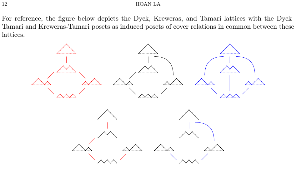
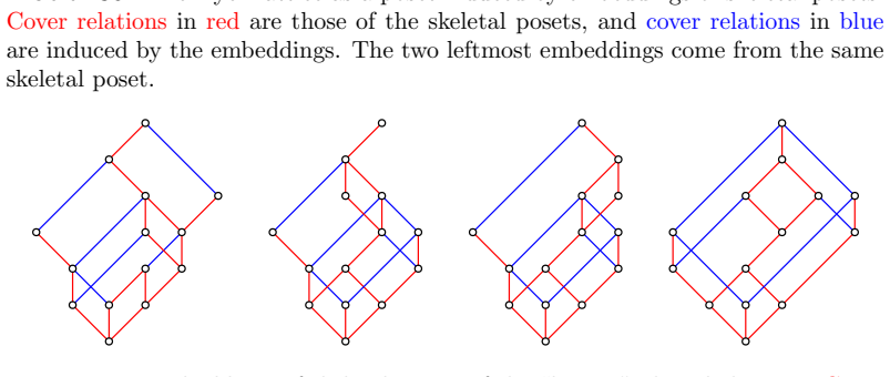
Altitude lattices within each family share the same number of linear intervals because they arise from a fixed distributive lattice and are connected by height-preserving extensions and refinements whose skeletal posets SK(L) embed into one another; SK(L) is the poset induced by the cover relations labeled 1 and its Hasse diagram is the largest spanning subgraph common to the Hasse diagrams of any two such related lattices.

What carries the argument

The skeletal poset SK(L) induced by the cover relations labeled 1, whose Hasse diagram supplies the largest common spanning subgraph between height-preserving lattice extensions.

If this is right

  • Every altitude lattice inside one family has the same count of linear intervals.
  • The skeletal posets of related lattices embed into one another under height-preserving extensions and refinements.
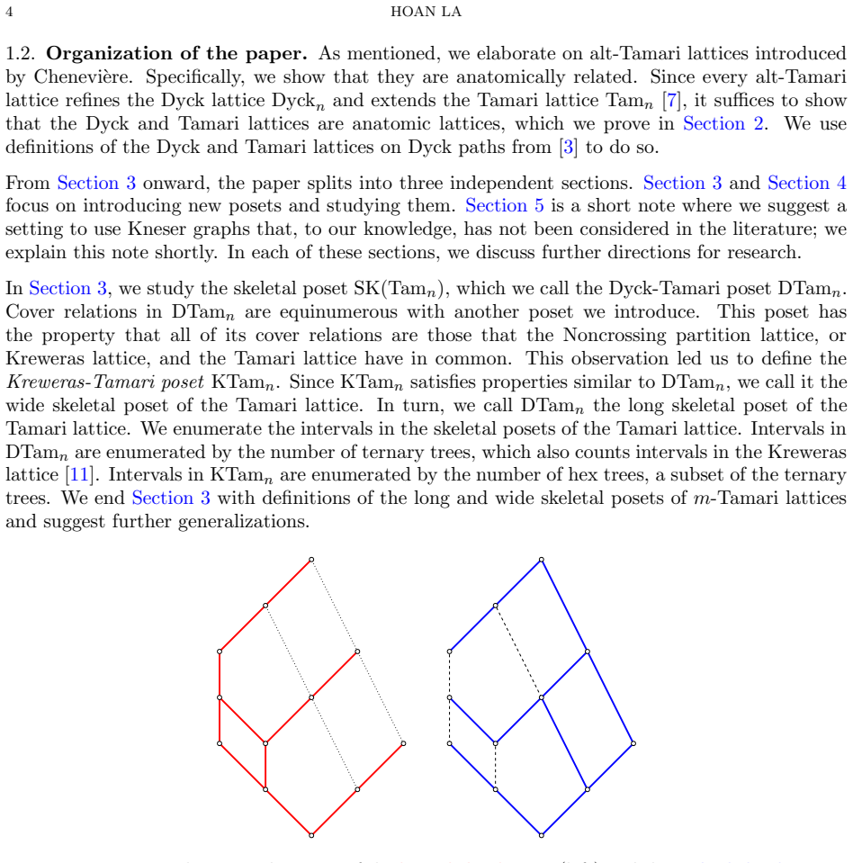
  • The number of intervals in SK(Tam_n) and its companion poset can be enumerated directly.
  • Kneser graphs KG(k) on the height-k elements of a poset with zero admit observations usable in reconstruction problems.

Where Pith is reading between the lines

These are editorial extensions of the paper, not claims the author makes directly.

  • The skeletal-poset construction may supply a uniform way to count linear intervals across any height-preserving lattice family.
  • The Kneser graphs defined on height slices could serve as invariants for deciding when two posets are isomorphic from their height-labeled structure alone.
  • The relation between altitude lattices and Tamari lattices may extend to other well-known distributive lattices and produce new enumerative identities.

Load-bearing premise

That the cover relations labeled 1 always induce a poset whose Hasse diagram is precisely the largest spanning subgraph shared by the Hasse diagrams of any two lattices that preserve element heights under extension.

What would settle it

Two altitude lattices from the same family whose numbers of linear intervals differ, or a pair of height-preserving extensions whose common cover relations labeled 1 do not form the claimed skeletal poset.

Figures

Figures reproduced from arXiv: 2606.17274 by Hoan La.

Figure 1
Figure 1. Figure 1: The interval [1, 6] in the posets (N, ≤) (left) and (N, |) (right). An interval I in P is denoted [x, y] := {z ∈ P : x ≤ z ≤ y}. A cover relation x ⋖ y is the interval [x, y] := {x, y}. The Hasse diagram of a poset P is a directed acyclic graph (S, ⋖) with edges x⋖y, and P is the reflexive transitive closure of its cover relations ⋖. 1 arXiv:2606.17274v1 [math.CO] 15 Jun 2026 [PITH_FULL_IMAGE:figures/full… view at source ↗
Figure 2
Figure 2. Figure 2: Examples of alt-Tamari lattices with the poset induced by cover relations in red. Elements are labeled with h(x↓) and cover relations x ⋖ y labeled with h(y↓)−h(x↓). The leftmost lattice extends the one to its right. The rightmost poset is the induced poset. Proof. (i) Let ˆ0 ⋖ z ⋖ ˆ1 be a chain in L. By definition of h, h(ˆ0 ⋖ z) = 1. Since h(L) = h(ˆ1↓) and h(ˆ0 ⋖ z) = h(z↓), it follows that h(z ⋖ ˆ1) = … view at source ↗
Figure 3
Figure 3. Figure 3: The Hasse diagrams of the long skeletal poset (left) and the wide skeletal poset (right) of the m-Tamari lattice (for m = 2) in red and blue respectively. · · · and −− are cover relations in the m-Tamari lattice. In Section 4, we introduce a generalization of the alt-Tamari lattices. Besides being anatomically related, alt-Tamari lattices have the same number of linear intervals, i.e., intervals that are c… view at source ↗
Figure 4
Figure 4. Figure 4: A family of altitude lattices. The lattice on the left side of an arrow is refine by the lattice on the right side of an arrow. The cover relations in red induce the skeletal poset of the rightmost lattice. • There are 7 elements or one-element chains. • There are 8 cover relations or two-element chains. • There are 5 intervals that are three-element or four-element chains, they are – for the leftmost latt… view at source ↗
Figure 5
Figure 5. Figure 5: A summary of the bijection between bracket vectors and Dyck paths below. For each paired u and d, there is an integer counting pairs of letters u and d between such a pair. The bracket vector here is (4, 0, 2, 0, 0) and the Dyck path here is u1u2d3u4u5d6u7d8d9d10. Proof. For v a bracket vector, we use vi for 1 ≤ i ≤ n to write a Dyck path w as follows: • let w := w1w2 · · · w2n be a word, and I := {1, 2, .… view at source ↗
Figure 6
Figure 6. Figure 6: u1u2d3d4u5u6d7d8 ⋖ u1u2d3u4d5u6d7d8 in Dyck4 [PITH_FULL_IMAGE:figures/full_fig_p007_6.png] view at source ↗
Figure 7
Figure 7. Figure 7: u1u2d3d4u5u6d7d8 ⋖ u1u2d3u4u5d6d7d8 in Tam4. By Theorem 2.6 and Theorem 2.7 with [PITH_FULL_IMAGE:figures/full_fig_p008_7.png] view at source ↗
Figure 8
Figure 8. Figure 8: u1u2d3d4u5d6u7d8 ⋖ u1u2d3d4u5u6d7d8 in DTam4. We end this section by counting cover relations in the Dyck-Tamari poset (for Section 3) using an idea of Galor and highlight a remark by Bj¨orner and Wachs (for Section 4; also see [PITH_FULL_IMAGE:figures/full_fig_p009_8.png] view at source ↗
Figure 9
Figure 9. Figure 9: The Dyck lattice Dyck4 (left) and the Tamari lattice Tam4 (right) as induced posets in the grid Z 3 ≥0 . Note the added 0 is for comparison with bracket vectors. Cover relations in red induce the Hasse diagram of the Dyck-Tamari poset DTam4; see Section 4 for further details. 3. Skeletal posets of Tamari lattices This section is independent of Section 4 and Section 5. The goal here is to study not one, but… view at source ↗
Figure 10
Figure 10. Figure 10: u1u2d3d4u5u6d7d8 ⋖ u1u2u3u4d5d6d7d8 in Krew4. When k = 1 in Theorem 3.1, we have AudDB⋖AuDdB. Similar to the Dyck-Tamari poset DTamn, cover relations AudDB ⋖AuDdB are cover relations that the Kreweras and Tamari lattices have in common. We call the poset induced by these cover relations the Kreweras-Tamari poset KTamn. Definition 3.2 (Kreweras-Tamari poset). The Kreweras-Tamari poset KTamn is the reflexiv… view at source ↗
Figure 11
Figure 11. Figure 11: u1d2u3d4u5u6d7d8 ⋖ u1d2u3u4u5d6d7d8 in KTam4. As mentioned, there are nCn cover relations AudDB⋖AuDdB in KTamn+1. Although we sketched a proof earlier, let us give a proof via a bijection between AudDB ⋖AuDdB and AdudB ⋖AuddB. Proposition 3.3 (A bijection between cover relations in the Dyck-Tamari poset and cover relations in the Kreweras-Tamari posets). There exists a bijection between cover relations Ad… view at source ↗
Figure 12
Figure 12. Figure 12: Left: u1u2d3d4, u1u2d3d4u5d6 ⋖ u1u2d3u4d5d6 in DTam3. Right: u1u2d3d4, u1d2u3u4d5d6 ⋖ u1u2u3d4d5d6 in KTam3. Proof. For any Dyck path w, there are n pairs of letters u and d as described in the bijection from Theorem 2.5. Consider such a pair of letters u and d. For u, we write AuduB. For d, we write AdudB. The second u, or the letter u as written in AuduB with a larger index, is paired with a letter d. T… view at source ↗
Figure 13
Figure 13. Figure 13: Top: The Dyck lattice Dyck3 in red (leftmost), the Tamari lattice Tam3 (middle), the Kreweras lattice KTam3 (rightmost). Bottom: The Dyck￾Tamari poset DTam3 (left) induced by cover relations in red and the Kreweras￾Tamari poset KTam3 (right) induced by cover relations in blue. 3.2. Properties of the Kreweras-Tamari poset. Although the Kreweras-Tamari poset KTamn is not a skeletal poset in the sense of The… view at source ↗
Figure 14
Figure 14. Figure 14: The interval [(2, 0, 0, 0),(2, 1, 0, 0)] in Tam4, and intervals [(0, 0),(1, 0)] and [(0),(0)] in Tam2 and Tam1, respectively. Proof. Consider an interval [v = (v1, v2, . . . , vn), v′ = (v ′ 1 , v′ 2 , . . . , v′ n )] in the Tamari lattice Tamn such that v1 = v ′ 1 = k. Recall from Theorem 2.5 that vi for 1 ≤ i ≤ n is the number of pairs of letters u and d between the i-th pair of letters u and d in Dyck … view at source ↗
Figure 15
Figure 15. Figure 15: The interval [(1, 0, 1, 0),(3, 0, 1, 0)] in Tam4, and intervals [0, 0] and [(1, 0),(1, 0)] in Tam1 and Tam2, respectively. Proof. Consider an interval [v = (v1, v2, . . . , vn), v′ = (v ′ 1 , v′ 2 , . . . , v′ n )] in the Tamari lattice Tamn such that v1 < v′ 1 = n − 1. Recall from Theorem 2.5 that vi for 1 ≤ i ≤ n counts the number of pairs of letters u and d between the i-th pair of letters u and d in D… view at source ↗
Figure 16
Figure 16. Figure 16: The interval [(3, 0, 0, 0, 1, 0, 0),(5, 1, 0, 2, 1, 0, 0)] in Tam7, and intervals [(0, 0),(1, 0)], [(0, 1, 0),(2, 1, 0)] and [(0),(0)] in Tam2, Tam3, and Tam1, respectively. Proof. The lemma follows from Theorem 3.7 and Theorem 3.8. It reduces to Theorem 3.7 if [MT, M′ ] is the empty interval, and to Theorem 3.8 if [R, R′ ] is the empty interval. □ Using Theorem 3.9, we can characterize intervals in the D… view at source ↗
Figure 17
Figure 17. Figure 17: The interval [(3, 0, 0, 0, 0, 0, 0),(5, 1, 0, 2, 1, 0, 0)] in DTam7, and intervals [(0, 0),(1, 0)], [(0, 0, 0),(2, 1, 0)] and [(0),(0)] in DTam2, DTam3, and DTam1, respectively. Proof. By Theorem 3.9, we can write any interval [w, w′ ] in DTamn as [uLM dT R, uL′M′dR′ ]. Recall from Theorem 2.13 that cover relations in DTamn are of the form AdudB⋖AuddB. Observe that there exists cover relations uLM dT R = … view at source ↗
Figure 18
Figure 18. Figure 18: The interval [u1d2u3d4u5u6d7d8, u1u2d3d4u5u6d7d8] in DTam4 where d4u5u6 is fixed. In terms of bracket vectors, the interval is [(0, 0, 1, 0),(1, 0, 1, 0)]. Theorem 3.11 is a comparability criterion for elements in DTamn. Since it is stated in terms of Dyck paths, we restate this criterion in terms of bracket vectors. Both versions are necessary for us to enumerate the intervals in DTamn. Corollary 3.12 (C… view at source ↗
Figure 19
Figure 19. Figure 19: The interval [(1, 0, 0, 0),(3, 0, 1, 0)] in DTam4 mapped to the interval [(1, 0, 0, 0, 0),(4, 3, 0, 1, 0)] in DTam5. Explicitly, for intervals in [uLM dT, uL′M′dR′ ] in DTamn−1, we map these intervals to [uLM dT ud, uuL′M′dR′d] that we rewrite as [uM dT, uM′d]. The intervals [uM dT, uM′d] are in DTamn given that they satisfy the condition in Theorem 3.13. We are left with intervals [w, w′ ] in DTamn−1 whe… view at source ↗
Figure 20
Figure 20. Figure 20: The interval [(3, 0, 1, 0, 0),(4, 0, 2, 1, 0)] in DTam5. Observe that (3, 0, 1, 0) ̸≤ (0, 2, 1, 0). Observe that intervals [(v1, v2, . . . , vn−1, 0),(n − 1, v′ 1 , v′ 2 , . . . , v′ n−1 )] includes those of the form [uLM dT, uLM′d] where the interval [L, L′ ] is nonempty. Specifically, if v2 = v ′ 1 in Theorem 3.14, then we have the interval [(v2, v3, . . . , vv1 ),(v ′ 1 , v′ 2 , . . . , vv1 )] in DTamv… view at source ↗
Figure 21
Figure 21. Figure 21: The bijection in the proof of Theorem 3.15. Proof. Before moving forward, we recommend that the reader keep in mind what was previously said right after Theorem 3.13 and after Theorem 3.14. By Theorem 3.13, it suffices to consider intervals [w, w′ ] = [u . . . duuE, u . . . duuE′ ] in DTamn−1 and intervals [uM dT, uM′d], where u k = u1u2 · · · uk for 2 ≤ k ≤ n − 2 and [Dmax, D′ max] is the largest interva… view at source ↗
Figure 22
Figure 22. Figure 22: The interval [(0, 0, 1, 0, 0),(3, 2, 1, 0, 0)] in KTam5, and intervals [(0, 1, 0),(2, 1, 0)] and [(0),(0)] in KTam3 and KTam1, respectively. Proof. By Theorem 3.7, if v1 = v ′ 1 , then an interval [v = (v1, v2, . . . , vn), v′ = (v ′ 1 , v′ 2 , . . . , v′ n )] in KTamn can be written as [uLdR, uL′dR′ ]. This is the case where the Dyck paths M, M′ , and T are empty. It suffices to show that if v1 < v′ 1 , … view at source ↗
Figure 23
Figure 23. Figure 23: The interval [(0, 0, 1, 0, 0),(3, 2, 1, 0, 0)] in KTam5 mapped to the interval [(0, 1, 0, 0, 0),(0, 3, 2, 1, 0, 0)] in DTam5. Consider AudDB in the cover relation AudDB ⋖ AuDdB in KTamn by Theorem 3.2. Let M be the mirror map defined as follows: for letters u and d in a Dyck path w, M : uk → d2n−k+1 and M : dk → u2n−k+1 for 1 ≤ k ≤ 2n. For example, M : u1d2u3u4d5d6 → u1u2d3d4u5d6. The idea is to transform… view at source ↗
Figure 24
Figure 24. Figure 24: An example of a 3-Dyck path. Since the m-Tamari lattice is an interval in the Tamari lattice restricted to m-Dyck paths, we do not need to (re)define it here. However, the same can not be said for the skeletal posets of the m￾Tamari lattice. To define these posets, we extend the bijection from Theorem 3.3. We recommend that the reader see [PITH_FULL_IMAGE:figures/full_fig_p020_24.png] view at source ↗
Figure 25
Figure 25. Figure 25: The bijection from Theorem 3.3 for 3-Dyck paths. Top: from a 3- Dyck path to a cover relation in 3-DTamn. Bottom: from a 3-Dyck path to a cover relation in 3-KTamn. In this case as depicted, they are the same. For a m-Dyck path w, we add u md m after a letter d as shown in the top half of [PITH_FULL_IMAGE:figures/full_fig_p020_25.png] view at source ↗
Figure 26
Figure 26. Figure 26: The Dyck lattice Dyck3 (left) and the Tamari lattice Tam3 (right) as intervals in some posets P and Q, respectively. −− indicate the existence of cover relations involving elements not in these intervals. ←→ indicates the maps between P and Q, i.e., refinement of P/extension of Q, involving c⋖d and c⋖e in red. In this figure, P and Q have the same number of linear intervals (see Theorem 4.1). Moving forwa… view at source ↗
Figure 27
Figure 27. Figure 27: Two examples of P and Q; each with an interval that is nonlinear in P but linear in Q [PITH_FULL_IMAGE:figures/full_fig_p023_27.png] view at source ↗
Figure 28
Figure 28. Figure 28: A small example of lattices with the same number of linear intervals. Our goal with Theorem 4.2 is to give a universal approach to extending or refining any poset P or Q. However, in practice, it may be overly tedious to check that p = q1 + q2 + q3. In an effort to convince the reader that our approach can be useful and interesting (for some posets P and Q), we use Theorem 4.2 to find lattices with the sa… view at source ↗
Figure 29
Figure 29. Figure 29: The Hasse diagrams of some lattices with the same number of linear intervals as the Dyck lattice (for n = 4). 4.3. Polygonal lattices in the grid. Formally, the lattices in [PITH_FULL_IMAGE:figures/full_fig_p025_29.png] view at source ↗
Figure 30
Figure 30. Figure 30: Smallest examples of P and Q embedded in the grid Z 2 ≥0 . Geometrically, observe that a cover relation corresponds to a line segment along an axis. Further￾more, the height h(x↓) for any element x is invariant under the refinements and extensions of P and Q, respectively. In certain cases, h(x↓) is the sum of coordinates of x in the grid. We mentioned earlier that they are ways of refining P or extending… view at source ↗
Figure 31
Figure 31. Figure 31: An extension/refinement forcing another in the grid embedding. By construction, we want P and Q to always be embeddable into the grid as described earlier with [PITH_FULL_IMAGE:figures/full_fig_p026_31.png] view at source ↗
Figure 32
Figure 32. Figure 32: P has less linear intervals than Q. Consider the figure above. Observe that the purple interval is nonlinear in P but is linear in Q. P has 4 linear intervals that are 3 element chains while Q has 5 of such linear intervals. This is an example where the grid allow us to ignore some undesirable cases as they are not realizable by construction. In general, it allow us to ignore linear intervals in products … view at source ↗
Figure 33
Figure 33. Figure 33: Two embeddings of the Dyck lattice in Z 3 ≥0 . 4.4. Extensions and refinements of the Dyck lattice in the grid. Now that we have the necessary setup, we focus on two examples. In each example, we refine the Dyck lattice to get lattices with the same number of linear intervals. Each sequence of refinements stops whenever it reaches a “largest” lattice (we use “largest” in the geometric sense, i.e., convex … view at source ↗
Figure 34
Figure 34. Figure 34: From the Dyck lattice to the Tamari lattice (for n = 4). A.I/B.I and A.III/B.IV are the Dyck and Tamari lattices, respectively. Below is the list of 14 linear intervals for each lattice; 12 linear intervals are 3 element chains and 2 linear intervals are 4 element chains. We recommend that the reader note the differences in linear intervals. I. The 3-element linear intervals are [a, g], [b, i], [b, g], [c… view at source ↗
Figure 35
Figure 35. Figure 35: From the Dyck lattice to a Cambrian lattice (see [PITH_FULL_IMAGE:figures/full_fig_p028_35.png] view at source ↗
Figure 36
Figure 36. Figure 36: The Dyck lattice as a poset induced by embeddings of skeletal posets. Cover relations in red are those of the skeletal posets, and cover relations in blue are induced by the embeddings. The two leftmost embeddings come from the same skeletal poset [PITH_FULL_IMAGE:figures/full_fig_p029_36.png] view at source ↗
Figure 37
Figure 37. Figure 37: Embeddings of skeletal posets of the “largest” altitude lattices. Cover relations in red are those of the skeletal posets, and cover relations in blue are induced by the embeddings. Every lattice in the above figures is realizable as a poset induced by embeddings of some skeletal posets, namely, the skeletal posets of the “largest” lattices. Motivated by alt-Tamari lattices, we say that these lattices bel… view at source ↗
Figure 38
Figure 38. Figure 38: Embeddings of SK(Tam4) with 4, 5 and 6 induced cover relations in blue from left to right, respectively. With the same setting as before, we consider a random embedding of a skeletal poset into the product of chains recorded by λ. Geometrically, recall that cover relations in this embedding correspond to line segments along some axes. For such an embedding, it is natural to count the minimal and maximal n… view at source ↗
read the original abstract

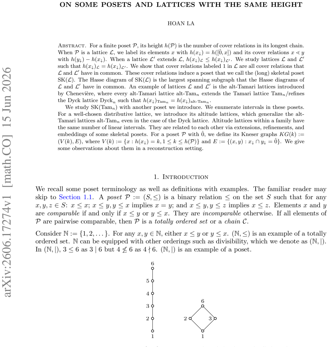
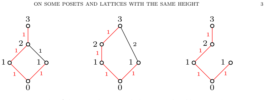
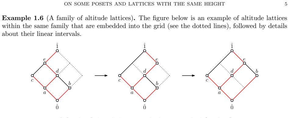
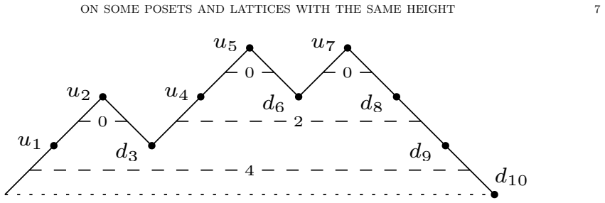
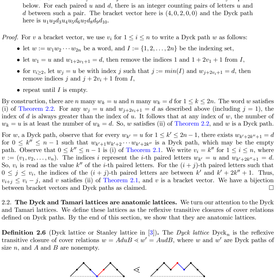
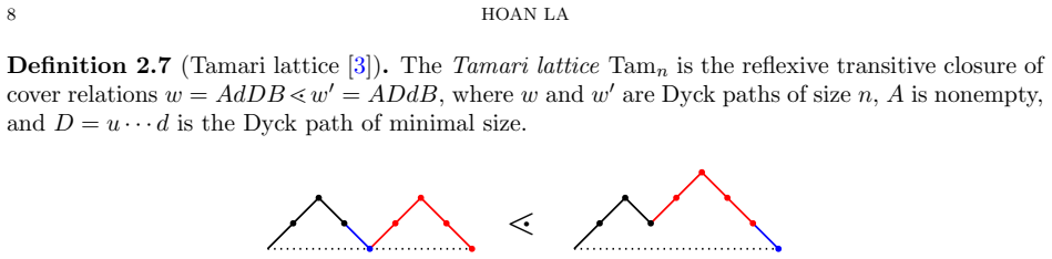
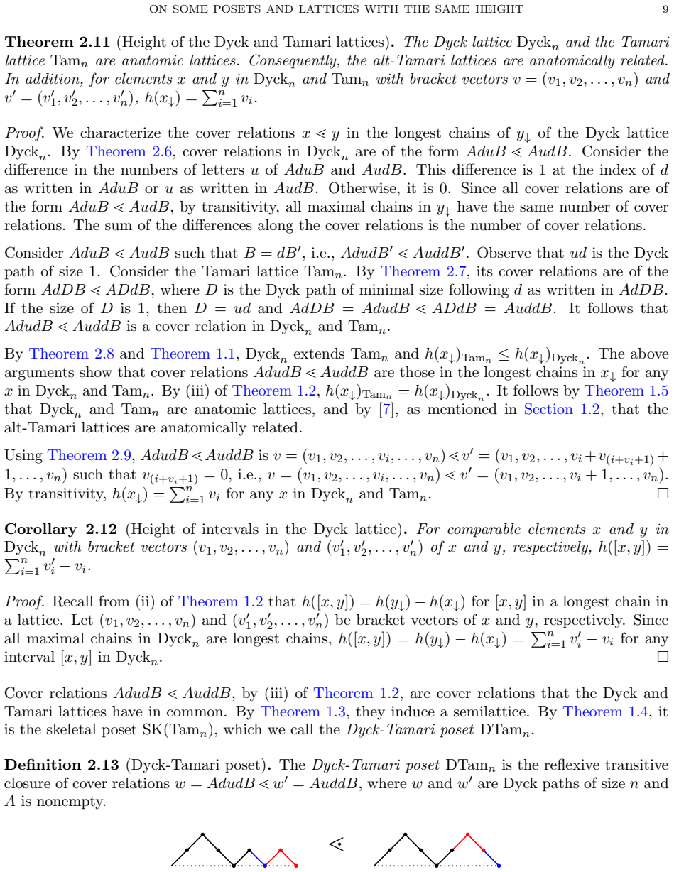
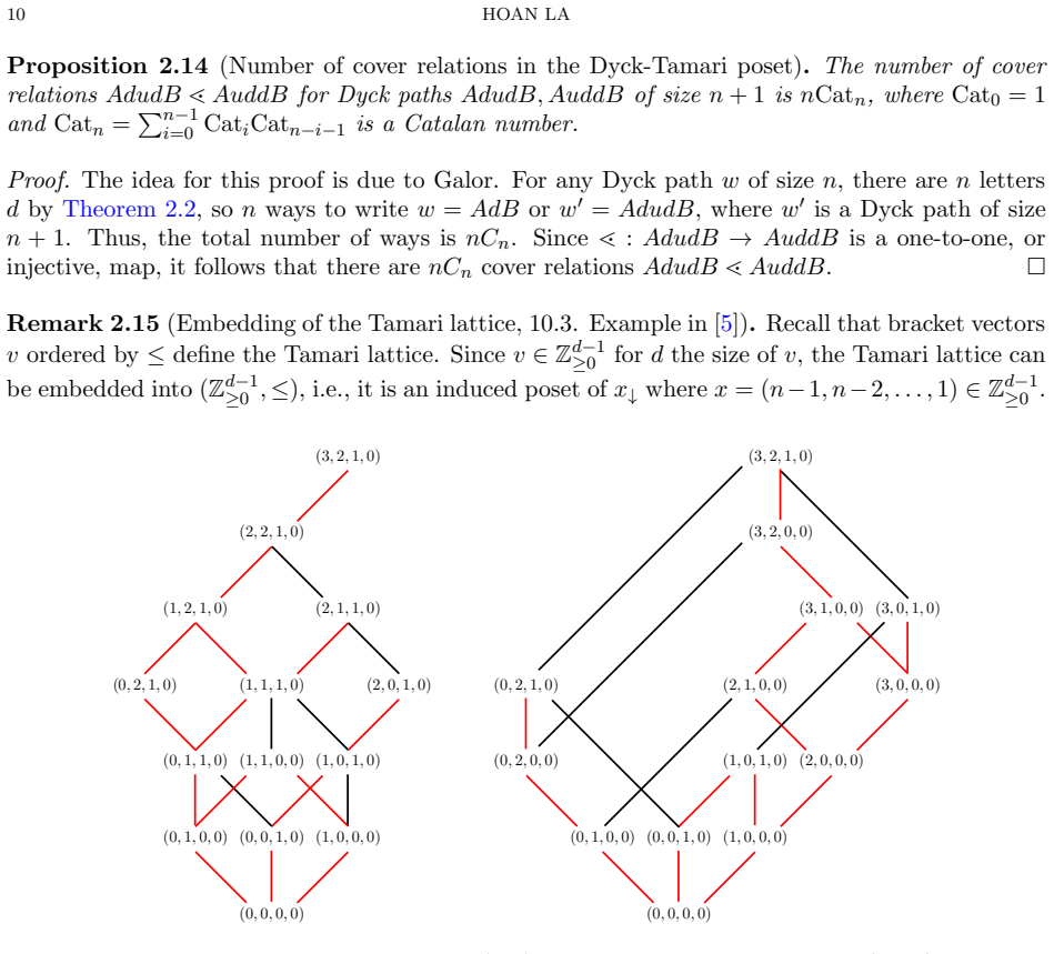
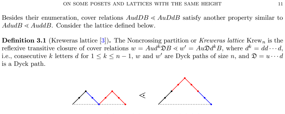
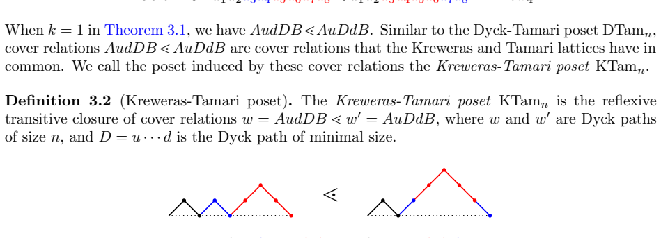
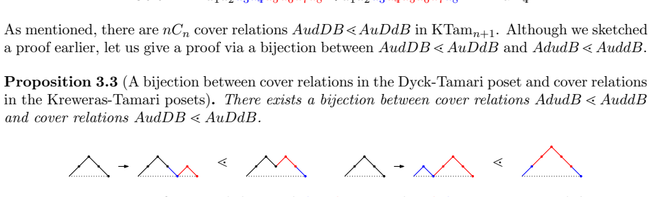
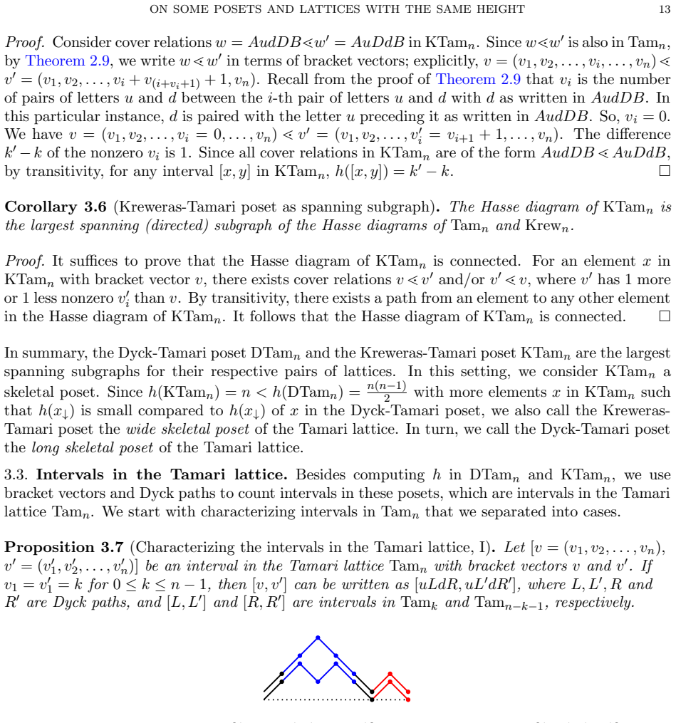
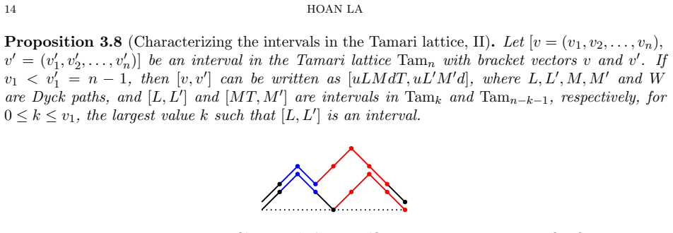
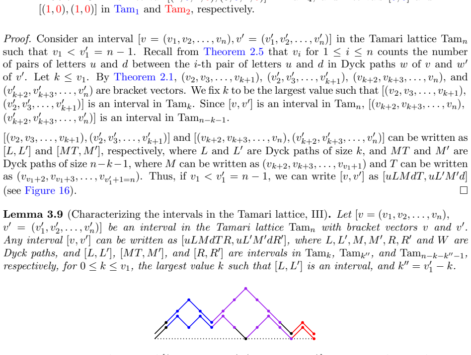
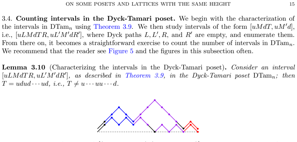
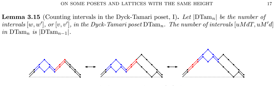
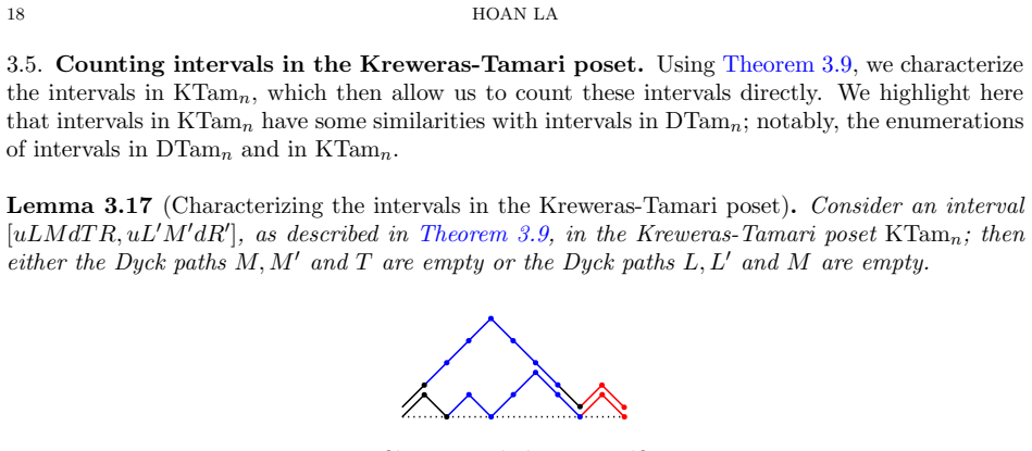
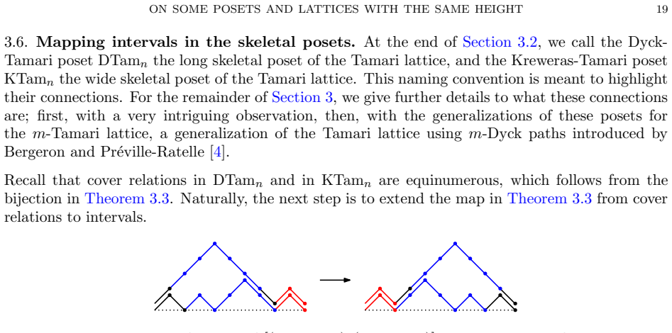
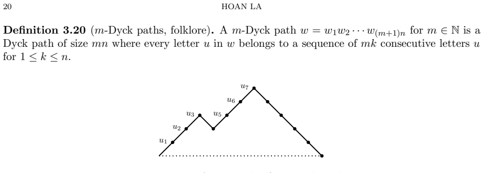
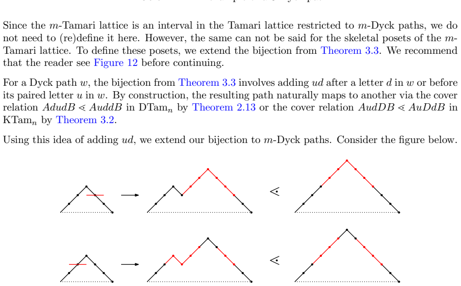
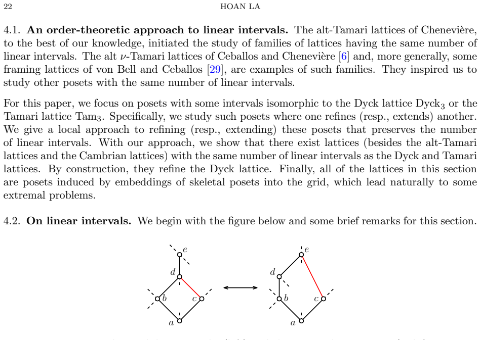
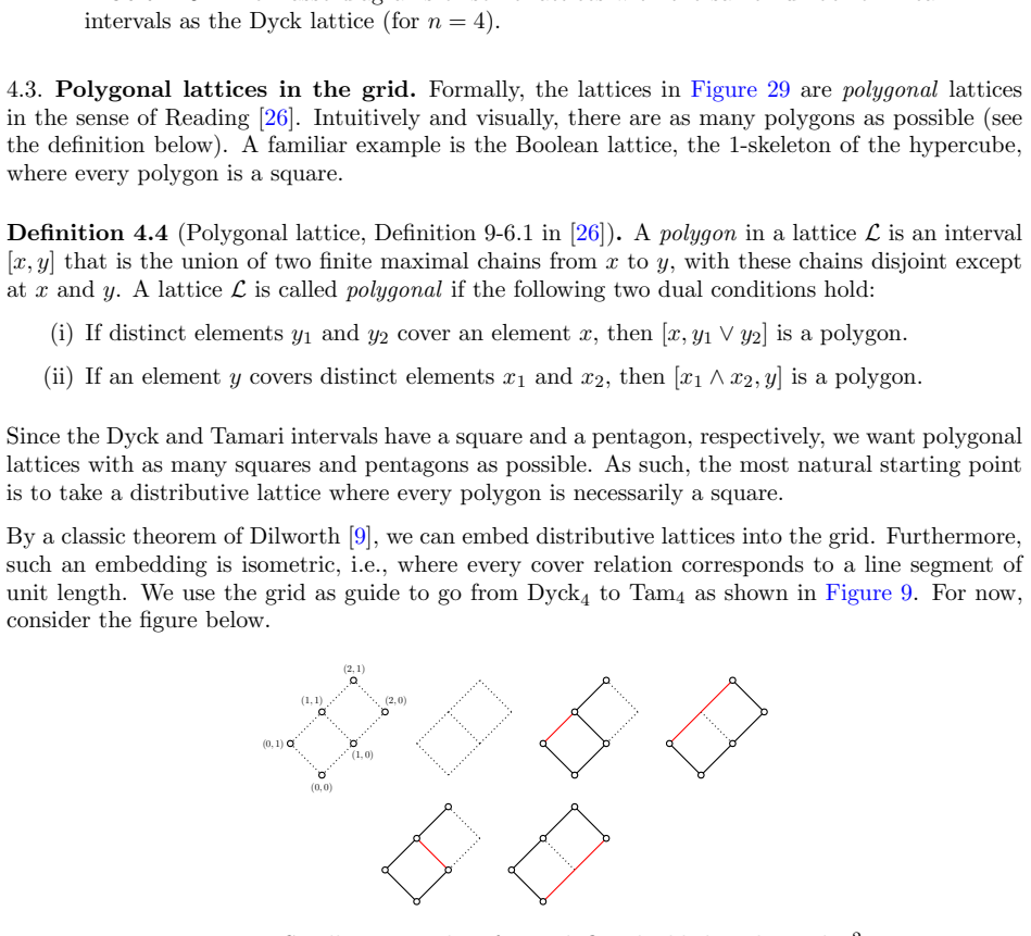
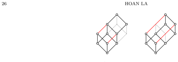
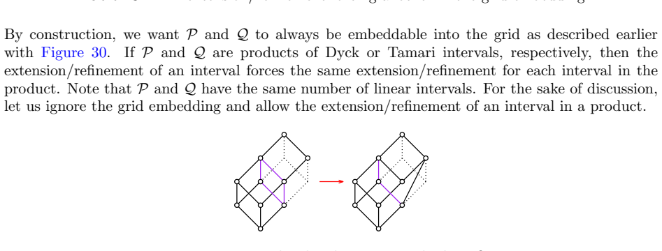
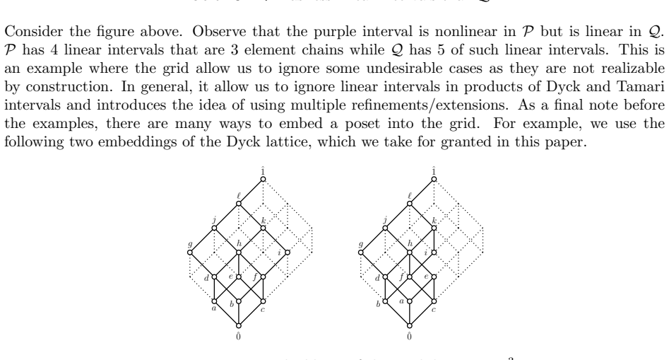
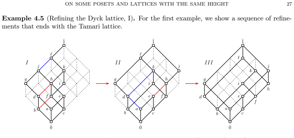
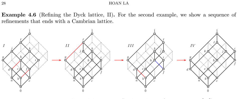
For a finite poset $\mathcal{P}$, its height $h(\mathcal{P})$ is the number of cover relations in its longest chain. When $\mathcal{P}$ is a lattice $\mathcal{L}$, we label its elements $x$ with $h(x_\downarrow) = h([\hat{0},x])$ and its cover relations $x \lessdot y$ with $h(y_\downarrow) - h(x_\downarrow)$. When a lattice $\mathcal{L}'$ extends $\mathcal{L}$, $h(x_\downarrow)_\mathcal{L} \leq h(x_\downarrow)_{\mathcal{L}'}$. We study lattices $\mathcal{L}$ and $\mathcal{L}'$ such that $h(x_\downarrow)_\mathcal{L} = h(x_\downarrow)_{\mathcal{L}'}$. Cover relations labeled $1$ in $\mathcal{L}$ induce a poset that we call the (long) skeletal poset $\mathrm{SK}(\mathcal{L})$. Its Hasse diagram is the largest spanning subgraph that the Hasse diagrams of $\mathcal{L}$ and $\mathcal{L}'$ have in common. An example of lattices $\mathcal{L}$ and $\mathcal{L}'$ is the alt-Tamari lattices introduced by Chenevi\`ere, where every alt-Tamari lattice $\mathrm{alt}\text{-}\mathrm{Tam}_n$ extends the Tamari lattice $\mathrm{Tam}_n$/refines the Dyck lattice $\mathrm{Dyck}_n$ such that $h(x_\downarrow)_{\mathrm{Tam}_n} = h(x_\downarrow)_{\mathrm{alt}\text{-}\mathrm{Tam}_n}$. We study $\mathrm{SK}(\mathrm{Tam}_n)$ with another poset we introduce. We enumerate intervals in these posets. For a well-chosen distributive lattice, we introduce its altitude lattices, which generalize the alt-Tamari lattices $\mathrm{alt}\text{-}\mathrm{Tam}_n$. Altitude lattices within a family have the same number of linear intervals. They are related to each other via extensions, refinements, and embeddings of some skeletal posets. For a poset $\mathcal{P}$ with $\hat{0}$, we define its Kneser graphs $KG(k) := (V(k),E)$, where $V(k) := \{x: h(x_\downarrow) = k, 1 \leq k \leq h(\mathcal{P})\}$ and $E := \{(x,y): x_\downarrow \cap y_\downarrow =\hat{0}\}$. We give some observations about them in a reconstruction setting.

Editorial analysis

A structured set of objections, weighed in public.

Desk editor's note, referee report, simulated authors' rebuttal, and a circularity audit. Tearing a paper down is the easy half of reading it; the pith above is the substance, this is the friction.

Referee Report

3 major / 2 minor

Summary. The manuscript defines the height of a poset and a labeling of elements and covers in a lattice by the height of the principal ideal. It considers pairs of lattices L and L' related by extension with identical height functions h(x_↓). From the label-1 covers it extracts a skeletal poset SK(L) whose Hasse diagram is asserted to be the largest common spanning subgraph of the Hasse diagrams of L and L'. The paper studies this construction for the Tamari, alt-Tamari and Dyck lattices, introduces a family of altitude lattices generalizing the alt-Tamari lattices, claims that all members of such a family have the same number of linear intervals, and relates them by extensions, refinements and embeddings of skeletal posets. It also defines Kneser graphs KG(k) on the rank-k elements of a poset with 0̂ and records observations about them in a reconstruction context.

Significance. If the invariance of the number of linear intervals and the embedding relations via skeletal posets can be established, the work would supply a new invariant and a uniform framework for comparing several well-studied lattice families. The definitional character of the manuscript, however, leaves the actual strength of these contributions dependent on the missing derivations.

major comments (3)
  1. [Abstract] Abstract (paragraph defining SK(L)): the claim that the Hasse diagram of SK(L) is the largest spanning subgraph common to Hasse(L) and Hasse(L') is asserted without proof. Height preservation alone does not immediately guarantee that every label-1 cover remains a cover in L' or that no higher-label edge of L becomes a cover in L'; a counter-example or a detailed argument is required because this identification is used to relate Tam_n, alt-Tam_n and Dyck_n and to construct the embeddings for the altitude-lattice family.
  2. [Altitude lattices] Section introducing altitude lattices: the statement that 'altitude lattices within a family have the same number of linear intervals' is presented as a theorem but no enumeration, recurrence, or bijection is supplied in the abstract or indicated in the text. Because this invariance is the central new claim, a self-contained proof or explicit computation for at least one non-trivial family is needed.
  3. [Kneser graphs] Section on Kneser graphs: the reconstruction observations are stated without any supporting lemma or example that would allow verification; if these observations are intended to illustrate the utility of the skeletal-poset construction, they must be tied explicitly to the earlier definitions.
minor comments (2)
  1. [Tamari and alt-Tamari study] The manuscript refers to 'another poset we introduce' when discussing SK(Tam_n) but does not name or define it; a short definition or reference to the relevant subsection would improve readability.
  2. [Definitions] Notation for the height function is overloaded (h(P) for the height of the poset and h(x_↓) for the height of an ideal); a brief clarification at first use would prevent confusion.

Simulated Author's Rebuttal

3 responses · 0 unresolved

We thank the referee for the careful reading and for identifying points where additional justification is needed. The manuscript is primarily definitional, and we agree that the central claims require explicit arguments. We will revise the text to supply the missing derivations while preserving the original scope.

read point-by-point responses
  1. Referee: [Abstract] Abstract (paragraph defining SK(L)): the claim that the Hasse diagram of SK(L) is the largest spanning subgraph common to Hasse(L) and Hasse(L') is asserted without proof. Height preservation alone does not immediately guarantee that every label-1 cover remains a cover in L' or that no higher-label edge of L becomes a cover in L'; a counter-example or a detailed argument is required.

    Authors: We acknowledge the need for a formal argument. The equality h(x_↓)_L = h(x_↓)_L' implies that any label-1 cover x ≺ y in L cannot admit an intermediate element z in L', because that would force h(z_↓) to lie strictly between the common values, contradicting the cover relation in L. Conversely, no cover of label greater than 1 in L can become a cover in L' without violating the shared height function. We will insert a short lemma (new Lemma 2.3) proving that the Hasse diagram of SK(L) is precisely the largest common spanning subgraph, together with a verification on the Tam_n / alt-Tam_n pair. revision: yes

  2. Referee: [Altitude lattices] Section introducing altitude lattices: the statement that 'altitude lattices within a family have the same number of linear intervals' is presented as a theorem but no enumeration, recurrence, or bijection is supplied in the abstract or indicated in the text. Because this invariance is the central new claim, a self-contained proof or explicit computation for at least one non-trivial family is needed.

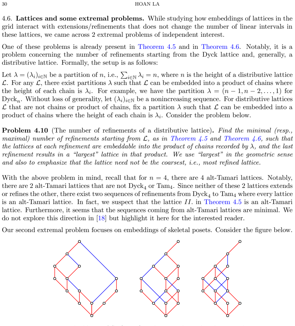
    Authors: The invariance follows from the fact that every linear interval in an altitude lattice projects onto a unique maximal chain in the common skeletal poset SK(L). We will add a bijection (new Proposition 4.5) showing that linear intervals are in one-to-one correspondence with saturated chains of SK(L) that avoid certain forbidden subposets; the count is therefore independent of the particular altitude lattice in the family. For the smallest non-trivial family we will also tabulate the numbers explicitly for n ≤ 6. revision: yes

  3. Referee: [Kneser graphs] Section on Kneser graphs: the reconstruction observations are stated without any supporting lemma or example that would allow verification; if these observations are intended to illustrate the utility of the skeletal-poset construction, they must be tied explicitly to the earlier definitions.

    Authors: We will expand the Kneser-graph section with a concrete example on the rank-2 elements of Tam_4, exhibiting the edges of KG(2) and showing how they correspond to pairs of principal ideals whose intersection is trivial precisely when the corresponding elements are incomparable in SK(Tam_4). A short lemma (new Lemma 5.2) will link the edge condition directly to the height labeling and the skeletal poset. revision: yes

Circularity Check

0 steps flagged

No significant circularity; paper is definitional and observational with independent constructions.

full rationale

The paper defines height labeling on lattices, introduces the skeletal poset SK(L) directly from cover relations labeled 1, and defines altitude lattices as a generalization of alt-Tamari lattices. Claims about shared linear-interval counts and relations via extensions/embeddings follow from these explicit constructions and standard height-preservation assumptions without reducing any result to a fitted parameter, self-citation chain, or renaming. No load-bearing self-citations appear; external references (e.g., to Chenevière) are to prior independent work. Enumeration of intervals and Kneser-graph observations are presented as direct consequences of the new objects rather than derived predictions. The derivation chain remains self-contained against external benchmarks.

Axiom & Free-Parameter Ledger

0 free parameters · 1 axioms · 2 invented entities

The central claims rest on standard order-theoretic definitions and the introduction of new combinatorial objects without additional free parameters or external evidence for the new entities.

axioms (1)
  • domain assumption For a lattice L' extending L, the height h(x_↓) in L is less than or equal to that in L'.
    Stated as a general property when introducing the study of lattices with equal heights.
invented entities (2)
  • skeletal poset SK(L) no independent evidence
    purpose: Induced poset from cover relations labeled 1, representing common Hasse diagram subgraph between L and L'.
    Newly defined to study the common structure between L and L'.
  • altitude lattice no independent evidence
    purpose: Generalization of alt-Tamari lattices for well-chosen distributive lattices preserving interval counts.
    Introduced as a new family with the stated properties.

pith-pipeline@v0.9.1-grok · 6012 in / 1722 out tokens · 79665 ms · 2026-06-27T02:34:23.223838+00:00 · methodology

discussion (0)

Sign in with ORCID, Apple, or X to comment. Anyone can read and Pith papers without signing in.

Reference graph

Works this paper leans on

29 extracted references · 1 linked inside Pith

  1. [1]

    The zero-divisor graph of a commutative semigroup: a survey.Groups, modules, and model theory - surveys and recent developments, Springer, 2017, 23–39

  2. [2]

    I. Beck. Coloring of commutative rings.J. Algebra,116(1988), 208–226

  3. [3]

    Bernardi, N

    O. Bernardi, N. Bonichon. Intervals in Catalan lattices and realizers of triangulations.J. Combin. Theory Ser.A, 116(2009), 55–75

  4. [4]

    Bergeron, L.-F

    F. Bergeron, L.-F. Pr´ eville-Ratelle. Higher trivariate diagonal harmonics via generalized Tamari posets.J. Comb., 3(2012), 317–341

  5. [5]

    Bj¨ orner, M

    A. Bj¨ orner, M. L. Wachs. Shellable nonpure complexes and posets. II.Trans. Amer. Math. Soc.,349(1997), 3945–3975

  6. [6]

    Ceballos, C

    C. Ceballos, C. Chenevi` ere. On linear intervals in the altν-Tamari lattices.Comb. Theory,4(2024)

  7. [7]

    Chenevi` ere

    C. Chenevi` ere. Linear intervals in the Tamari and the Dyck lattices and in the alt-Tamari posets.Preprint, arXiv:2209.00418

  8. [8]

    Chˆ atel, V

    G. Chˆ atel, V. Pilaud. Cambrian Hopf algebras.Adv. Math.,311(2017), 598–633

  9. [9]

    R. P. Dilworth. A decomposition theorem for partially ordered sets.Ann. of Math, (2)51(1950), 161–166

  10. [10]

    H. R. Daneshpajouh, F. Meunier. Box complexes: at the crossroad of graph theory and topology.Discrete Math, 348(2025)

  11. [11]

    P. H. Edelman. Chain enumeration and noncrossing partitions.Discrete Math.,31(1980), 171–180

  12. [12]

    Godsil, K

    C. Godsil, K. Meagher. Erd¨ os-Ko-Rado theorems: algebraic approaches. Cambridge Studies in Advanced Math- ematics, 149.Cambridge University Press, Cambridge, (2016)

  13. [13]

    Halaˇ s, M

    R. Halaˇ s, M. Jukl. On Beck’s coloring of posets.Discrete Math.,309(2009), 4584–4589

  14. [14]

    Huang, D

    S. Huang, D. Tamari. Problems of associativity: A simple proof for the lattice property of systems ordered by a semi-associative law.J. Combinatorial Theory Ser. A,13(1972), 7–13

  15. [15]

    Kneser, Aufgabe 300,Jber

    M. Kneser, Aufgabe 300,Jber. Deutsch. Math.-Verein.,58(1955)

  16. [16]

    D. J. Kleitman, B. I. Rothschild. Asymptotic enumeration of partial orders on a finite set.Trans. Amer. Math. Soc.,205(1975), 205–220

  17. [17]

    H. La. Skeletal posets of Tamari lattices.In preparation

  18. [18]

    H. La. On linear intervals and altitude lattices.In preparation

  19. [19]

    Lov´ asz

    L. Lov´ asz. Kneser’s conjecture, chromatic number, and homotopy.J. Combin. Theory Ser. A,25(1978), 319–324

  20. [20]

    Merino, T

    A. Merino, T. M¨ utze, and Namrata. Kneser graphs are Hamiltonian.Adv. Math.,468(2025)

  21. [21]

    R. H. M¨ ohring. Almost all comparability graphs are UPO.Discrete Math.,50(1984), 63–70

  22. [22]

    M¨ uller-Hoissen, J

    F. M¨ uller-Hoissen, J. M. Pallo, and J. Stasheff, editors. Associahedra, Tamari Lattices and Related Structures. Tamari Memorial Festschrift, volume 299 ofProgress in Mathematics. Springer, New York, 2012

  23. [23]

    (2026), The On-Line Encyclopedia of Integer Sequences, Published electronically athttps: //oeis.org

    OEIS Foundation Inc. (2026), The On-Line Encyclopedia of Integer Sequences, Published electronically athttps: //oeis.org

  24. [24]

    V. Pons. Combinatorics of the Permutahedra, Associahedra, and Friends. Habilitation ` a diriger des recherches. Universit´ e Paris-Saclay, 2023

  25. [25]

    N. Reading. Cambrian lattices.Adv. Math.,205(2006), 313–353

  26. [26]

    N. Reading. Lattice theory of the poset of regions.Lattice theory: special topics and applications. Vol.2, 399–487, Birkh¨ auser/Springer, Cham, 2016

  27. [27]

    R. P. Stanley. Catalan numbers.Cambridge University Press,New York, 2015

  28. [28]

    D. Tamari. Monoides Pr´ eordonn´ es et Chaˆ ınes de Malcev (Ph.D. thesis), Universit´ e Paris Sorbonne, 1951

  29. [29]

    von Bell, C

    M. von Bell, C. Ceballos. Framing lattices and flow polytopes.Preprint, arXiv:2512.20575. Email address:hoan.la.work@gmail.com