Approximation and interactive design with exact 3D elastic curves
Pith reviewed 2026-06-26 15:44 UTC · model grok-4.3
The pith
An 11-parameter family from the spherical pendulum equation fully describes 3D elastic curve segments.
A machine-rendered reading of the paper's core claim, the machinery that carries it, and where it could break.
Core claim
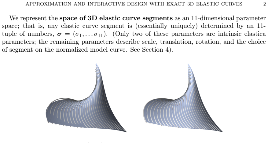
An analytic representation equivalent to the spherical pendulum equation leads to an 11-parameter description of the space of 3D elastic curve segments. Numerically stable methods recover the parameters from a given elastic curve segment and approximate arbitrary space curve segments by 3D elasticas.
What carries the argument
The 11-parameter family of 3D elastic curve segments obtained by reduction to the spherical pendulum equation.
If this is right
- A numerically stable method recovers the 11 parameters from any given elastic curve segment.
- Arbitrary space curve segments admit fast stable approximation by 3D elasticas.
- Interactive design can employ exact elastic curves rather than approximate ones.
- CAD surfaces admit rationalization by elastic curves suitable for robotic hot-blade cutting.
Where Pith is reading between the lines
- The same reduction may supply a practical test for whether a measured physical rod is behaving as a true elastica.
- The approximation procedure could be inserted into existing CAD pipelines to enforce physical fairness constraints on free-form curves.
- Extensions to closed elastic curves or curves with fixed endpoints and tangents would follow directly from the same 11-parameter set.
- Comparison of the recovered parameters against measured torsion and curvature profiles on real elastic materials would give a direct experimental check.
Load-bearing premise
That every critical point of the bending energy for space curves is captured inside this single 11-parameter family without extra independent constraints or singular cases outside it.
What would settle it
A space curve that satisfies the Euler-Lagrange equation for bending energy yet lies outside every member of the 11-parameter family would falsify the claim of completeness.
Figures
read the original abstract
An elastic space curve is a critical point of the bending energy subject to appropriate constraints. An analytic representation, equivalent to the spherical pendulum equation, leads to an 11-parameter description of the space of 3D elastic curve segments. We give a numerically stable method for recovering the 11 parameters from a given elastic curve segment. Using this, we give a fast and stable method to approximate an arbitrary space curve segment by a 3D elastica. Applications include interactive design with exact elastic curves and CAD surface rationalization for robotic hot-blade cutting.
Editorial analysis
A structured set of objections, weighed in public.
Referee Report
Summary. The manuscript claims that an analytic representation equivalent to the spherical pendulum equation yields an 11-parameter description of the space of 3D elastic curve segments. It provides a numerically stable method to recover these parameters from a given elastic curve segment and a fast stable method to approximate arbitrary space curve segments by 3D elastica, with applications to interactive design and CAD surface rationalization for robotic hot-blade cutting.
Significance. If the 11-parameter family is complete for all critical points of the bending energy and the numerical methods are stable, the work would provide a practical analytic tool for exact elastic curves in design and manufacturing, potentially improving precision over purely numerical approaches in geometric modeling.
major comments (1)
- [Abstract] Abstract: The central claim that the spherical pendulum reduction exhaustively parametrizes every solution to the Euler-Lagrange equations for the 3D bending energy (yielding precisely 11 independent parameters) requires explicit demonstration that planar elastica and degenerate cases (e.g., vanishing curvature or aligned conserved quantities) do not require additional parameters or separate treatment; this completeness is load-bearing for the 11-parameter description.
minor comments (2)
- The abstract asserts numerical stability without reference to error analysis, convergence rates, or test cases; these should be added to support the recovery and approximation methods.
- Notation for the 11 parameters and the mapping from the spherical pendulum should be introduced with clear definitions early in the manuscript to aid readability.
Simulated Author's Rebuttal
We thank the referee for their careful reading and for identifying a point where the completeness argument can be made more explicit. We address the single major comment below.
read point-by-point responses
-
Referee: [Abstract] Abstract: The central claim that the spherical pendulum reduction exhaustively parametrizes every solution to the Euler-Lagrange equations for the 3D bending energy (yielding precisely 11 independent parameters) requires explicit demonstration that planar elastica and degenerate cases (e.g., vanishing curvature or aligned conserved quantities) do not require additional parameters or separate treatment; this completeness is load-bearing for the 11-parameter description.
Authors: The reduction begins from the full Euler-Lagrange system for the bending energy of framed space curves and uses the three conserved quantities (energy and two components of angular momentum) to obtain the spherical-pendulum ODE. All solutions of the original system are recovered this way; the planar elastica arise precisely when the angular-momentum vector is aligned with a principal axis of the curve or when the azimuthal momentum vanishes, reducing the pendulum to a great-circle motion. Straight lines and circles appear as equilibrium or separatrix solutions of the same pendulum equation. The eleven parameters are the three position coordinates, three orientation angles, the four pendulum constants (energy, two angular-momentum components, integration phase), and the scaling factor for arc length; no additional parameters are introduced by the special cases. We nevertheless agree that an explicit verification subsection would remove any ambiguity and will insert one in the revised manuscript. revision: partial
Circularity Check
No circularity; 11-parameter family follows from external spherical pendulum equivalence
full rationale
The paper states that an analytic representation 'equivalent to the spherical pendulum equation' leads to the 11-parameter description of 3D elastic curve segments. This equivalence is a known result in the elastica literature and is not derived or fitted inside the paper. No self-citation is invoked as load-bearing for the completeness claim, no parameters are fitted to data and then relabeled as predictions, and no ansatz or uniqueness theorem is smuggled via prior author work. The recovery and approximation methods are numerical procedures built on top of the representation rather than circular reductions. The derivation chain is therefore self-contained against external benchmarks.
Axiom & Free-Parameter Ledger
axioms (1)
- domain assumption The Euler-Lagrange equation for the bending energy of a space curve is equivalent to the spherical pendulum equation.
Reference graph
Works this paper leans on
-
[1]
Carlo Alessi, Camilla Agabiti, Daniele Caradonna, Cecilia Laschi, Federico Renda, and Egidio Falotico, Rod models in continuum and soft robot control: a review, arXiv preprint arXiv:2407.05886 (2024)
Pith/arXiv arXiv 2024
-
[2]
Olivier Ameline, Sinan Haliyo, Xingxi Huang, and Jean AH Cognet,Classifications of ideal 3d elastica shapes at equilibrium, Journal of Mathematical Physics58(2017), no. 6
2017
-
[3]
3, 1728–1748
Costanza Armanini, Fr´ ed´ eric Boyer, Anup Teejo Mathew, Christian Duriez, and Federico Renda,Soft robots modeling: A structured overview, IEEE Transactions on Robotics39(2023), no. 3, 1728–1748
2023
-
[4]
a solution construction procedure, Journal of Elasticity139(2020), no
Josu J Arroyo, ´Oscar J Garay, and ´Alvaro P´ ampano,Boundary value problems for euler-bernoulli planar elastica. a solution construction procedure, Journal of Elasticity139(2020), no. 2, 359–388
2020
-
[5]
Milan Batista,Elfun18–a collection of matlab functions for the computation of elliptic integrals and jacobian elliptic functions of real arguments, SoftwareX10(2019), 100245
2019
-
[6]
Mikl´ os Bergou, Max Wardetzky, Stephen Robinson, Basile Audoly, and Eitan Grinspun,Discrete elastic rods, ACM Siggraph 2008 Papers, 2008, pp. 1–12
2008
-
[7]
Minghao Bi, Yunzhen He, Zhi Li, Ting-Uei Lee, and Yi Min Xie,Design and construction of kinetic structures based on elastica strips, Automation in Construction146(2023), 104659
2023
-
[8]
Brander, J
D. Brander, J. Gravesen, and T. Nørbjerg,Approximation by planar elastic curves, Adv. Comput. Math. (2016)43(2016), 25–43
2016
-
[9]
David Brander, Jakob Andreas Bærentzen, Kenn Clausen, Ann-Sofie Fisker, Jens Gravesen, Morten N Lund, Toke Bjerge Nørbjerg, Kasper Hornbak Steenstrup, and Asbjørn Søndergaard,Designing for hot- blade cutting: geometric approaches for high-speed manufacturing of doubly-curved architectural surfaces, Advances in architectural geometry (AAG 2016), vdf Hochsc...
2016
-
[10]
David Brander, Jakob Andreas Bærentzen, Ann-Sofie Fisker, and Jens Gravesen,B´ ezier curves that are close to elastica, Computer-Aided Design104(2018), 36–44
2018
-
[11]
,Designing interactively with elastic splines, Computer Aided Geometric Design62(2018), 181– 191
2018
-
[12]
1, 13–26
Bille C Carlson,Numerical computation of real or complex elliptic integrals, Numerical Algorithms10 (1995), no. 1, 13–26
1995
-
[13]
4, 3483–3490
Andrew Choi, Ran Jing, Andrew P Sabelhaus, and Mohammad Khalid Jawed,Dismech: A discrete differential geometry-based physical simulator for soft robots and structures, IEEE Robotics and Au- tomation Letters9(2024), no. 4, 3483–3490
2024
-
[14]
2, 73–85
Pierre Cuvilliers, Justina R Yang, Lancelot Coar, and Caitlin Mueller,A comparison of two algorithms for the simulation of bending-active structures, International Journal of Space Structures33(2018), no. 2, 73–85. APPROXIMATION AND INTERACTIVE DESIGN WITH EXACT 3D ELASTIC CUR VES 20
2018
-
[15]
4, 905–923
C´ atia da Costa e Silva, Sascha F Maassen, Paulo M Pimenta, and J¨ org Schr¨ oder,A simple finite element for the geometrically exact analysis of bernoulli–euler rods, Computational Mechanics65(2020), no. 4, 905–923
2020
-
[16]
thesis, 2019
Ann-Sofie Fisker,Surface design and rationalization for robotic hot-blade cutting, Ph.D. thesis, 2019
2019
-
[17]
Christian Hafner and Bernd Bickel,The design space of plane elastic curves, ACM Transactions on Graphics (TOG)40(2021), no. 4, 1–20
2021
-
[18]
4, 441–460
Berthold KP Horn,The curve of least energy, ACM Transactions on Mathematical Software (TOMS)9 (1983), no. 4, 441–460
1983
-
[19]
2, 5687–5694
Shiyu Jin, Wenzhao Lian, Changhao Wang, Masayoshi Tomizuka, and Stefan Schaal,Robotic cable routing with spatial representation, IEEE Robotics and Automation Letters7(2022), no. 2, 5687–5694
2022
-
[20]
2, 86–97
Carlos L´ azaro, Juan Bessini, and Salvador Monle´ on,Mechanical models in computational form finding of bending-active structures, International Journal of Space Structures33(2018), no. 2, 86–97
2018
-
[21]
2020, International Association for Shell and Spatial Structures (IASS), 2020, pp
Ting-Uei Lee and Yi Min Xie,From ruled surfaces to elastica-ruled surfaces: new possibilities for creating architectural forms, Proceedings of IASS Annual Symposia, vol. 2020, International Association for Shell and Spatial Structures (IASS), 2020, pp. 1–12
2020
-
[22]
A Levin, I Grinberg, ED Rimon, and A Shapiro,Dual arm steering of flexible linear objects in 2-d and 3-d environments using euler’s elastica solutions, IEEE Robotics and Automation Letters (2025)
2025
-
[23]
4, 625–636
Mark Moll and Lydia E Kavraki,Path planning for deformable linear objects, IEEE Transactions on Robotics22(2006), no. 4, 625–636
2006
-
[24]
7558–7564
Andrea Monguzzi, Niccol` o Mantegna, Andrea Maria Zanchettin, and Paolo Rocco,Potential field-based online path planning for robust cable routing, 2024 IEEE/RSJ International Conference on Intelligent Robots and Systems (IROS), IEEE, 2024, pp. 7558–7564
2024
-
[25]
Abhyankar’s 60th Birthday Conference, Springer, 1994, pp
David Mumford,Elastica and computer vision, Algebraic Geometry and its Applications: Collections of Papers from Shreeram S. Abhyankar’s 60th Birthday Conference, Springer, 1994, pp. 491–506
1994
-
[26]
Toke Bjerge Nørbjerg,Rationalization in architecture with surfaces foliated by elastic curves, (2017)
2017
-
[27]
2, 269–291
Karthikeyan Panneerselvam, Rahul, and Suvranu De,A constrained spline dynamics (csd) method for interactive simulation of elastic rods, Computational mechanics65(2020), no. 2, 269–291
2020
-
[28]
9, 4253–4264
Kiril P Petkov and Jesper H Hattel,Hot-blade cutting of eps foam for double-curved surfaces—numerical simulation and experiments, The International Journal of Advanced Manufacturing Technology93 (2017), no. 9, 4253–4264
2017
-
[29]
Ulrich Pinkall and Oliver Gross,Differential geometry: From elastic curves to willmore surfaces, Springer Nature, 2024
2024
-
[30]
2, 564–592
Jianhong Shen, Sung Ha Kang, and Tony F Chan,Euler’s elastica and curvature-based inpainting, SIAM journal on Applied Mathematics63(2003), no. 2, 564–592
2003
-
[31]
1002, Citeseer, 2008, p
David A Singer,Lectures on elastic curves and rods, AIP Conference Proceedings, vol. 1002, Citeseer, 2008, p. 3
2008
-
[32]
Asbjørn Søndergaard, Jelle Feringa, Toke Nørbjerg, Kasper Steenstrup, David Brander, Jens Graversen, Steen Markvorsen, Andreas Bærentzen, Kiril Petkov, Jesper Hattel, et al.,Robotic hot-blade cutting: an industrial approach to cost-effective production of double curved concrete structures, Robotic fabrication in architecture, art and design 2016, Springer...
2016
-
[33]
1, 25–34
Saimir Tola, Alfred Daci, and Gentian Zavalani,A simulation of an elastic filament using kirchhoff model, Mathematics and Statistics10(2022), no. 1, 25–34
2022
-
[34]
Department of Applied Mathematics and Computer Science, Technical University of Den- mark, Richard Petersens Plads, Building 324, DK-2800, Kgs
Zhujiang Wang, Marco Fratarcangeli, Annie Ruimi, and AR Srinivasa,Real time simulation of inex- tensible surgical thread using a kirchhoff rod model with force output for haptic feedback applications, International Journal of Solids and Structures113(2017), 192–208. Department of Applied Mathematics and Computer Science, Technical University of Den- mark,...
2017
discussion (0)
Sign in with ORCID, Apple, or X to comment. Anyone can read and Pith papers without signing in.