REVIEW 2 major objections 8 minor 41 references
Exact vs approximate second-order derivatives in vertically-integrated ice sheet models
T0 review · 2 major / 8 minor · reviewed 2026-07-05 · glm-5.2
Pith's one-line read Approximate ice-sheet Hessian breaks after 4 modes
desk verdict Paper derives a second-order self-adjoint (SOSA) approximation for SSA ice sheet Hessians and benchmarks it spectrally against AD. The derivation is clean, the comparison is rigorous, and the conclusions are appropriately cautious. The main limitation is generalizability from two idealized domains. read the letter →
The pith
A machine-rendered reading of the paper's core claim, the machinery that carries it, and where it could break.
The reading
What carries the argument
The central objects are the SOSA (second-order self-adjoint) Hessian and the AD (algorithmic differentiation) Hessian for the SSA momentum balance. The comparison tool is principal angle analysis between eigenvector subspaces: the cosine of each principal angle is obtained from the SVD of the matrix formed by the inner products of the two sets of eigenvectors. Small angles mean the subspaces are nearly parallel; π/2 means orthogonal. The eigenvalue ratio of ~3 is traced to the Glen's flow law exponent n=3 entering the viscosity derivative.
What would settle it
If, on a domain with different flow regime (e.g., strong shear or grounding-line dynamics), the eigenvector subspaces were to diverge immediately at mode 1 rather than mode 4, the 'first 4 modes are safe' conclusion would not generalize.
Extended reading notes
Core claim
The central discovery is a quantitative characterization of how the self-adjoint approximation degrades second-order derivative information. The divergence is not catastrophic—the eigenvector subspaces start close and the divergence does not accelerate after approximately 50 modes—but it is real and structurally significant. The factor-of-3 eigenvalue compression traces directly to the Glen's law exponent, providing a mechanistic explanation for the systematic underestimation of curvature. The subspace alignment pattern (good for 4 modes, orthogonal by mode 33, stable thereafter) also retrospectively explains why first-order self-adjoint gradient methods have worked well in practice: there's
Load-bearing premise
The self-adjoint approximation assumes that the tangent linear operator of the SSA residual is self-adjoint, which holds only when the vertically-averaged effective viscosity is treated as independent of ice velocity. This is false for Glen's flow law with n=3, where viscosity depends nonlinearly on the strain rate and hence on velocity. The entire SOSA derivation and the resulting spectral comparison depend on this linearization.
Editorial extensions
If this is right
- Ice sheet models using SOSA for Newton-type optimisation should expect reliable curvature information only in the first 3-4 search directions, with progressively degraded directions beyond that.
- For Bayesian uncertainty quantification requiring the inverse Hessian for posterior covariance, SOSA will systematically underestimate uncertainty in every direction by roughly a factor of 3, and the eigenvector misalignment beyond mode 4 makes faithful covariance reconstruction unlikely without thousands of modes.
- The factor-of-n eigenvalue compression suggests a simple scaling correction could partially rescue SOSA for leading-mode applications, though the subspace divergence limits its effectiveness at higher rank.
- The subspace alignment pattern provides a retrospective explanation for the empirical success of self-adjoint approximations in first-order ice sheet inverse problems: gradient methods explore curvature directions sequentially, and the first few are the ones that matter most.
Reading between the lines
- The 'first 4 modes are safe' threshold is established on only two synthetic domains. Domains with stronger shear margins, grounding-line proximity, or different flow regimes could shift this threshold in either direction—particularly if nonlinear viscosity terms contribute more to the Hessian structure in those settings.
- The factor-of-3 eigenvalue ratio is tied to n=3 (Glen's law). If a different rheological exponent were used, the ratio would scale accordingly, suggesting the eigenvalue compression is a predictable structural feature rather than a domain-specific artifact.
- The persistent orthogonal subspace after mode 33 suggests there exists a class of curvature directions that are entirely invisible to the self-adjoint approximation—directions driven by velocity-dependent viscosity feedbacks. Identifying what physical structures these eigenvectors correspond to could guide when the approximation is safe versus dangerous.
- The methodology (principal angle analysis between approximate and exact Hessians) is generalizable beyond ice sheets to any PDE-constrained optimisation where a self-adjoint approximation is used, and could serve as a diagnostic tool for assessing approximation fidelity in other geophysical inverse problems.
Editorial analysis
A structured set of objections, weighed in public.
Referee Report
Summary. This manuscript derives a second-order self-adjoint (SOSA) formulation for the shallow-stream approximation (SSA) of ice sheet flow, in which the nonlinear dependence of viscosity on velocity is neglected (the standard linear-viscosity approximation). The resulting approximate Hessian-vector products are compared against exact Hessians computed via algorithmic differentiation (AD) in a JAX-based finite-volume code. The comparison uses two synthetic test domains (an ice shelf and a snaking ice stream) and employs spectral diagnostics—eigenvalue residuals, orthogonality residuals, and principal angles between invariant subspaces—to quantify the fidelity of the approximation. The main finding is that the SOSA and AD Hessians share similar leading eigenvector structure for approximately the first 4 modes, after which the subspaces diverge, with SOSA eigenvalues systematically smaller by a factor of roughly 3. The authors conclude that the SOSA Hessian is case-dependent in utility and recommend the full AD Hessian where high-fidelity second-order information is needed above very low rank.
Significance. The paper addresses a practically important question for the ice sheet modeling community: whether the widely used self-adjoint (linear-viscosity) approximation, well-established for first-order adjoints, can be extended to second-order derivatives with acceptable fidelity. The derivation (Appendices A–B) is self-contained and follows standard adjoint methodology cleanly. The spectral comparison is rigorous: eigenvalue residuals (Eq. 20) and orthogonality residuals (Eq. 21) confirm numerical quality of both Hessians, and principal angles between subspaces provide a principled similarity metric. The implementation in JAX enables a clean AD ground truth. The finding that subspace divergence begins after approximately 4 modes and the eigenvalue ratio of ~3 are concrete, falsifiable results that provide actionable guidance to practitioners. The honest assessment—that the approximation is case-dependent and inferior to the full Hessian above low rank—is appropriately cautious.
major comments (2)
- §5.2, paragraph on the factor-of-3 eigenvalue ratio: the heuristic explanation that '∂uG is roughly a factor of n=3 smaller when derivatives of the viscosity are included' is stated without derivation or reference. This is a load-bearing claim because it is the primary physical explanation for the systematic eigenvalue discrepancy that motivates the recommendation against using SOSA for uncertainty quantification (§6.2). A more precise justification—showing how the viscosity nonlinearity enters ∂uG and why it produces a factor of n in the eigenvalues—should be provided, or the claim should be softened to a conjecture.
- §5.2 and §7: the conclusion that subspaces are safe 'up to the first 4 modes' is established on exactly two idealized domains, both with uniform thickness and no grounding line. The abstract and conclusion state this threshold as a general finding. Given that real ice sheet inverse problems involve grounding zones, variable thickness, and thermomechanical coupling, the generalizability of the '4 modes' threshold is a correctness-risk concern. The authors should add a brief statement in the conclusion acknowledging that the threshold is domain-specific and may shift under different flow regimes, or alternatively test a third domain with non-uniform thickness to strengthen the claim.
minor comments (8)
- Abstract: 'second order derivatives' and 'second-order derivatives' are both used; please unify hyphenation throughout.
- §4.1, Ice Shelf description: 'righ-hand-side' should be 'right-hand-side' (missing 't').
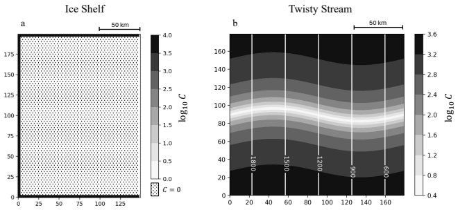
- §4.1, Twisty Stream: the formula for C contains nested parentheses that are hard to parse; please verify the closing delimiters match.
- Figure 5 caption: panels (a) and (b) labels in the caption text appear swapped relative to the figure layout described; please check consistency.
- §5.2: the introduction of the functional J in Eq. (19) comes after results from a different functional (J = ∫√(u·u)) are shown in §5.1; a brief note that the functional changes between subsections would help the reader.
- Eq. (9): the definition φ(q) = φ₀e^q is used without specifying the meaning of φ₀ or the units/dimensions of q; a brief clarification would help.
- Appendix B.2: the list of 9 terms (Eqs. B.11–B.19) is introduced as '12 terms' earlier in the text; please reconcile the count.
- §6.1: 'indetically zero' should be 'identically zero' (also appears in Appendix B.1, Eq. B.6 description).
Simulated Author's Rebuttal
We thank the referee for a careful and constructive report. Both major comments are well-taken and will be addressed in revision. On the factor-of-3 eigenvalue ratio, we agree the heuristic explanation is insufficiently justified and will either provide a more precise derivation or soften the claim to a conjecture. On the generalizability of the '4 modes' threshold, we agree it is domain-specific and will add an explicit caveat in the conclusion.
read point-by-point responses
-
Referee: §5.2, paragraph on the factor-of-3 eigenvalue ratio: the heuristic explanation that '∂uG is roughly a factor of n=3 smaller when derivatives of the viscosity are included' is stated without derivation or reference. This is a load-bearing claim because it is the primary physical explanation for the systematic eigenvalue discrepancy that motivates the recommendation against using SOSA for uncertainty quantification (§6.2). A more precise justification—showing how the viscosity nonlinearity enters ∂uG and why it produces a factor of n in the eigenvalues—should be provided, or the claim should be softened to a conjecture.
Authors: The referee is correct that the factor-of-3 explanation as currently stated is a heuristic assertion without sufficient justification. We will revise this in one of two ways. Our preferred approach is to provide a more precise derivation: the SSA effective viscosity scales as |u|^{(1-n)/n} under Glen's law, so the derivative of viscosity with respect to velocity introduces a factor of (1-n)/n, which for n=3 yields a factor of -2/3. The way this factor enters the operator ∂uG, combined with the structure of the Hessian-vector product (Eq. 17), can plausibly account for the observed ratio. However, we acknowledge that a fully rigorous derivation showing this factor propagates unchanged into the eigenvalues is not straightforward, as it depends on which terms dominate in each eigenmode. If we cannot complete this derivation to our satisfaction, we will instead soften the claim to a conjecture, explicitly stating that the factor-of-3 ratio is consistent with the viscosity nonlinearity scaling but that a rigorous derivation is not provided. Either way, the recommendation in §6.2 against using SOSA for uncertainty quantification does not depend solely on this explanation—it rests on the observed eigenvalue discrepancy itself, which is an empirical result from the spectral comparison. revision: partial
-
Referee: §5.2 and §7: the conclusion that subspaces are safe 'up to the first 4 modes' is established on exactly two idealized domains, both with uniform thickness and no grounding line. The abstract and conclusion state this threshold as a general finding. Given that real ice sheet inverse problems involve grounding zones, variable thickness, and thermomechanical coupling, the generalizability of the '4 modes' threshold is a correctness-risk concern. The authors should add a brief statement in the conclusion acknowledging that the threshold is domain-specific and may shift under different flow regimes, or alternatively test a third domain with non-uniform thickness to strengthen the claim.
Authors: We agree that the '4 modes' threshold is established on only two idealized domains and should not be stated as a general finding without qualification. We will add an explicit caveat in both the abstract and the conclusion acknowledging that this threshold is domain-specific and may shift under different flow regimes, particularly in the presence of grounding zones, variable thickness, or thermomechanical coupling. We considered adding a third test domain with non-uniform thickness, but we feel this is beyond the scope of a minor revision and would not by itself resolve the generalizability question—two or three idealized domains cannot establish a universal threshold. The honest and appropriate response is to qualify the claim rather than to overstate it. We will also adjust the language in §5.2 to make clear that the threshold of approximately 4 modes is specific to the Twisty Stream domain and that the broader, more robust finding is that subspace divergence begins at low rank and does not accelerate thereafter. revision: yes
Circularity Check
No circularity: the SOSA derivation is self-contained and validated against an independent AD-computed Hessian benchmark
full rationale
The paper derives a second-order self-adjoint (SOSA) approximation for the SSA ice sheet equations and compares its Hessian against an independently computed AD Hessian. The self-adjoint approximation (Eq. A.12) is explicitly stated as a modeling choice — freezing the viscosity μ̄ so that G is linear in u — and is the central object of study, not a concealed premise. No parameters are fitted to make the comparison work; the factor-of-3 eigenvalue ratio emerges from Glen's exponent n=3 in the physics, not from calibration. The spectral comparison (principal angles, eigenvalue residuals, orthonormality checks) uses standard linear algebra diagnostics applied to two independently constructed matrices. The derivation chain (Appendices A–B) proceeds from standard variational calculus: the Lagrangian (A.4) yields the FOA system (A.8), differentiation yields the SOA system (B.9–B.10), and the self-adjoint approximation simplifies terms but does not define the result in terms of itself. Citations are to external literature (MacAyeal, Cacuci, Petra et al., etc.) for standard adjoint methodology, not to a self-citation chain that would be load-bearing. The paper's conclusions (divergence after ~4 modes, eigenvalue ratio ~3, case-dependent utility) are empirical findings from the comparison, not definitions restated as predictions.
Assumptions & free parameters
free parameters (2)
- Glen's flow law exponent n =
3
- Domain geometry and slipperiness fields =
Ice Shelf: 500m uniform thickness, C=0 or 10^4; Twisty Stream: 1km thickness, C formula with epsilon=5e-3, R=180km, m=1/
assumptions (4)
- domain assumption Self-adjoint approximation: (∂uG(u))*[λ] = G(λ), i.e., the tangent linear operator of the SSA residual is self-adjoint
- domain assumption Functional J is separable in u and q, so ∂q∂uJ = 0
- standard math Standard first- and second-order adjoint methodology (Lagrange multiplier approach for PDE-constrained optimization)
- domain assumption Boundary conditions on adjoint variables match those on the forward variables, causing boundary terms from integration by parts to vanish
Cite this review
Pith. "Pith review of Exact vs approximate second-order derivatives in vertically-integrated ice sheet models." pith.science (2026). https://pith.science/paper/HOEYZGNC
@misc{pith2026260623691,
  author       = {Pith},
  title        = {Pith review of: Exact vs approximate second-order derivatives in vertically-integrated ice sheet models},
  year         = {2026},
  howpublished = {\url{https://pith.science/paper/HOEYZGNC}},
  note         = {Machine review of arXiv:2606.23691}
}
read the original abstract
Second order derivatives of model outputs with respect to input parameters are key to several applications in ice sheet modelling. For example, the ability to compute Hessian-vector products broadens the list of available optimisation methods, and facilitates certain kinds of parametric uncertainty quantification. Some modern ice sheet models are built on frameworks supporting algorithmic differentiation (AD), allowing for the computation of higher order derivatives with relative ease. However, many of our most widely-used models are not. A natural alternative might be to follow common practise in first order gradient computation and construct an approximate second-order adjoint model at the PDE level, which neglects the nonlinear dependence of ice viscosity on velocity. Here, we present such a model for the shallow-stream approximation allowing one to compute approximate second-order derivatives, and compare with full second-order derivates found using AD. We find that this produces Hessian-vector products that are superficially similar to those computed via AD. However, an analysis of the spectral decomposition of the Hessians calculated in each way reveals that the subspaces spanned by their eigenvectors diverge after the leading 4 modes, though divergence does not accelerate after this. We conclude that the utility of the approximate Hessian is case-dependent, and a full Hessian, likely computed using AD, should be used where high fidelity is required above very low rank.
Figures


Figures from the paper (2 more)


Reference graph
Works this paper leans on
-
[1]
H. Seroussi, S. Nowicki, E. Simon, A. Abe-Ouchi, T. Albrecht, J. Brondex, S.Cornford, C. Dumas, F. Gillet-Chaulet, H.Goelzer, N.R. Golledge, J. M. Gregory, R. Greve, M. J. Hoffman, A. Humbert, P. Huybrechts, T. Kleiner, E.Larour, G.Leguy, W.H.Lipscomb, D.Lowry, M.Mengel, M.Morlighem, F. Pattyn, A. J. Payne, D. Pollard, S. F. Price, A. Quiquet, T. J. Reeri...
-
[2]
D. R. MacAyeal, A tutorial on the use of control methods in ice-sheet modeling, Journal of Glaciology 39 (131) (1993) 91–98.doi:10.3189/ S0022143000015744
work page 1993
-
[3]
V. Rommelaere, D. R. MacAyeal, Large-scale rheology of the ross ice shelf, antarctica, computed by a control method, Annals of Glaciology 24 (1997) 43–48.doi:10.3189/S0260305500011915
- [4]
-
[5]
I. Joughin, D. R. MacAyeal, S. Tulaczyk, Basal shear stress of the ross ice streams from control method inversions, Journal of Geo- physical Research: Solid Earth 109 (B9) (2004).arXiv:https:// agupubs.onlinelibrary.wiley.com/doi/pdf/10.1029/2003JB002960, doi:https://doi.org/10.1029/2003JB002960. URLhttps://agupubs.onlinelibrary.wiley.com/doi/abs/10.1029/...
-
[6]
E. Larour, E. Rignot, I. Joughin, D. Aubry, Rheology of the ronne ice shelf, antarctica, inferred from satellite radar interferometry data using an inverse control method, Geophysical Research Letters 32 (5) (2005).arXiv:https://agupubs.onlinelibrary.wiley.com/doi/pdf/ 10.1029/2004GL021693,doi:https://doi.org/10.1029/2004GL021693. URLhttps://agupubs.onlin...
-
[7]
I.Joughin, S.Tulaczyk, J.L.Bamber, D.Blankenship, J.W.Holt, T.Scam- bos, D. G. Vaughan, Basal conditions for pine island and thwaites glaciers, west antarctica, determined using satellite and airborne data, Journal of Glaciology 55 (190) (2009) 245–257.doi:10.3189/002214309788608705
-
[8]
M. Morlighem, E. Rignot, H. Seroussi, E. Larour, H. Ben Dhia, D. Aubry, Spatial patterns of basal drag inferred using control methods from a full- stokes and simpler models for pine island glacier, west antarctica, Geo- physicalResearchLetters37(14)(2010).doi:https://doi.org/10.1029/ 2010GL043853
work page 2010
Show all 41 references
-
[9]
S. L. Cornford, D. F. Martin, A. J. Payne, E. G. Ng, A. M. Le Brocq, R. M. Gladstone, T.L.Edwards, S.R.Shannon, C.Agosta, M.R.vandenBroeke, H. H. Hellmer, G. Krinner, S. R. M. Ligtenberg, R. Timmermann, D. G. Vaughan, Century-scale simulations of the response of the west antar...
2015 doi
-
[10]
D. N. Goldberg, P. Heimbach, Parameter and state estimation with a time- dependent adjoint marine ice sheet model, The Cryosphere 7 (6) (2013) 1659–1678.doi:10.5194/tc-7-1659-2013. URLhttps://tc.copernicus.org/articles/7/1659/2013/
2013 doi
-
[11]
Larour, J
E. Larour, J. Utke, B. Csatho, A. Schenk, H. Seroussi, M. Morlighem, E. Rignot, N. Schlegel, A. Khazendar, Inferred basal friction and surface mass balance of the northeast greenland ice stream using data assimilation of icesat (ice cloud and land elevation satellite) surface ...
2014 doi
-
[12]
C. P. Koziol, J. A. Todd, D. N. Goldberg, J. R. Maddison, fenics_ice 1.0: a framework for quantifying initialization uncertainty for time-dependent ice sheet models, Geoscientific Model Development 14 (9) (2021) 5843–5861. doi:10.5194/gmd-14-5843-2021. URLhttps://gmd.copernicu...
2021 doi
-
[13]
R.M.Errico, Whatisanadjointmodel?, BulletinoftheAmericanMeteoro- logical Society 78 (11) (1997) 2577 – 2592.doi:10.1175/1520-0477(1997) 078<2577:WIAAM>2.0.CO;2
1997 doi
-
[14]
Marshall, A
J. Marshall, A. Adcroft, C. Hill, L. Perelman, C. Heisey, A finite-volume, incompressible navier stokes model for studies of the ocean on parallel computers, Journal of Geophysical Research: Oceans 102 (C3) (1997) 5753–5766.arXiv:https://agupubs.onlinelibrary.wiley.com/doi/ pd...
1997 doi
-
[15]
Giering, T
R. Giering, T. Kaminski, Recipes for adjoint code construction, ACM Trans. Math. Softw. 24 (4) (1998) 437–474.doi:10.1145/293686.293695. URLhttps://doi.org/10.1145/293686.293695
1998 doi
-
[16]
Heimbach, C
P. Heimbach, C. Hill, R. Giering, Automatic generation of efficient adjoint code for a parallel navier-stokes solver, in: P. M. A. Sloot, A. G. Hoekstra, C. J. K. Tan, J. J. Dongarra (Eds.), Computational Science — ICCS 2002, Springer Berlin Heidelberg, Berlin, Heidelberg, 200...
2002 doi
-
[17]
Heimbach, V
P. Heimbach, V. Bugnion, Greenland ice-sheet volume sensitivity to basal, surface and initial conditions derived from an adjoint model, Annals of Glaciology 50 (52) (2009) 67–80.doi:10.3189/172756409789624256. 17
2009 doi
-
[18]
Griewank, A
A. Griewank, A. Walther, Evaluating derivatives: principles and techniques of algorithmic differentiation, SIAM, 2008
2008
-
[19]
A. Hück, C. Bischof, M. Sagebaum, N. R. Gauger, B. Jurgelucks, E. Larour, G. Perez, A usability case study of algorithmic differentiation tools on the issm ice sheet model, Optimization Methods and Software 33 (4-6) (2018) 844–867.doi:10.1080/10556788.2017.1396602
2018 doi
-
[20]
URLhttps://gmd.copernicus.org/articles/14/4593/2021/
D.R.Shapero, J.A.Badgeley, A.O.Hoffman, I.R.Joughin, icepack: anew glacier flow modeling package in python, version 1.0, Geoscientific Model Development 14 (7) (2021) 4593–4616.doi:10.5194/gmd-14-4593-2021. URLhttps://gmd.copernicus.org/articles/14/4593/2021/
2021 doi
-
[21]
J. L. Lions, Optimal control of systems governed by partial differential equations, Vol. 170, Springer, 1971
1971
-
[22]
D. N. Goldberg, O. V. Sergienko, Data assimilation using a hybrid ice flow model, The Cryosphere 5 (2) (2011) 315–327.doi:10.5194/ tc-5-315-2011
2011
-
[23]
Martin, J
N. Martin, J. Monnier, Adjoint accuracy for the full stokes ice flow model: limits to the transmission of basal friction variability to the surface, The Cryosphere 8 (2) (2014) 721–741.doi:10.5194/tc-8-721-2014
2014 doi
-
[24]
Morlighem, H
M. Morlighem, H. Seroussi, E. Larour, E. Rignot, Inversion of basal friction in antarctica using exact and incomplete adjoints of a higher-order model, Journal of Geophysical Research: Earth Surface 118 (3) (2013) 1746–1753. doi:https://doi.org/10.1002/jgrf.20125
2013 doi
-
[25]
W. C. Thacker, Fitting models to inadequate data by enforc- ing spatial and temporal smoothness, Journal of Geophysical Re- search: Oceans 93 (C9) (1988) 10655–10665.arXiv:https://agupubs. onlinelibrary.wiley.com/doi/pdf/10.1029/JC093iC09p10655,doi: https://doi.org/10.1029/JC0...
1988 doi
-
[26]
W. C. Thacker, The role of the hessian matrix in fitting models to measure- ments, Journal of Geophysical Research: Oceans 94 (C5) (1989) 6177–6196. doi:https://doi.org/10.1029/JC094iC05p06177
1989 doi
-
[27]
Petra, J
N. Petra, J. Martin, G. Stadler, O. Ghattas, A computational frame- work for infinite-dimensional bayesian inverse problems, part ii: Stochas- tic newton mcmc with application to ice sheet flow inverse problems, SIAM Journal on Scientific Computing 36 (4) (2014) A1525–A1555.do...
2014 doi
-
[28]
Recinos, D
B. Recinos, D. Goldberg, J. R. Maddison, J. Todd, A framework for time-dependent ice sheet uncertainty quantification, applied to three west 18 antarctic ice streams, The Cryosphere 17 (10) (2023) 4241–4266.doi: 10.5194/tc-17-4241-2023. URLhttps://tc.copernicus.org/articles/17...
2023 doi
-
[29]
Recinos, D
B. Recinos, D. Goldberg, N. Gourmelen, J. R. Maddison, Mapping ice stream sensitivity in the amundsen sector to uncertainty in ice velocity observations, Geophysical Research Letters 52 (17) (2025) e2025GL117666, e2025GL117666 2025GL117666.arXiv:https:// agupubs.onlinelibrary....
2025 doi
-
[30]
D. G. Cacuci, Second-order adjoint sensitivity analysis methodology (2nd-asam) for computing exactly and efficiently first- and second- order sensitivities in large-scale linear systems: I. computational methodology, Journal of Computational Physics 284 (2015) 687–699. doi:htt...
2015 doi
-
[31]
D. G. Cacuci, The second-order adjoint sensitivity analysis methodology for nonlinear systems—i: Theory, Nuclear Science and Engineering 184 (1) (2016) 16–30.doi:10.13182/NSE16-16
2016 doi
-
[32]
Petra, H
N. Petra, H. Zhu, G. Stadler, T. J. Hughes, O. Ghattas, An inexact gauss- newton method for inversion of basal sliding and rheology parameters in a nonlinear stokes ice sheet model, Journal of Glaciology 58 (211) (2012) 889–903.doi:10.3189/2012JoG11J182
2012 doi
-
[33]
Isaac, N
T. Isaac, N. Petra, G. Stadler, O. Ghattas, Scalable and efficient algorithms forthepropagationofuncertaintyfromdatathroughinferencetoprediction for large-scale problems, with application to flow of the antarctic ice sheet, Journal of Computational Physics 296 (2015) 348–368.d...
2015 doi
-
[34]
H. Zhu, N. Petra, G. Stadler, T. Isaac, T. J. R. Hughes, O. Ghattas, Inversion of geothermal heat flux in a thermomechanically coupled non- linear stokes ice sheet model, The Cryosphere 10 (4) (2016) 1477–1494. doi:10.5194/tc-10-1477-2016
2016 doi
-
[35]
Necula, A
J.Bradbury, R.Frostig, P.Hawkins, M.J.Johnson, C.Leary, D.Maclaurin, G. Necula, A. Paszke, J. VanderPlas, S. Wanderman-Milne, Q. Zhang, JAX: composable transformations of Python+NumPy programs (2018). URLhttp://github.com/jax-ml/jax
2018
-
[36]
S. L. Cornford, D. F. Martin, D. T. Graves, D. F. Ranken, A. M. Le Brocq, R. M. Gladstone, A. J. Payne, E. G. Ng, W. H. Lipscomb, Adaptive mesh, finite volume modeling of marine ice sheets, Journal of Computational 19 Physics 232 (1) (2013) 529–549.doi:10.1016/j.jcp.2012.08.03...
2013 doi
-
[37]
D. R. MacAyeal, Large-scale ice flow over a viscous basal sediment: The- ory and application to ice stream b, antarctica, Journal of Geophysical Research: Solid Earth 94 (B4) (1989) 4071–4087.doi:https://doi.org/ 10.1029/JB094iB04p04071
1989 doi
-
[38]
Balay, S
S. Balay, S. Abhyankar, M. F. Adams, S. Benson, J. Brown, P. Brune, K. Buschelman, E. M. Constantinescu, L. Dalcin, A. Dener, V. Eijkhout, J. Faibussowitsch, W. D. Gropp, V. Hapla, T. Isaac, P. Jolivet, D. Karpeev, D. Kaushik, M. G. Knepley, F. Kong, S. Kruger, D. A. May, L. C...
2025
-
[39]
P. R. Amestoy, I. S. Duff, J.-Y. L’Excellent, J. Koster, A fully asynchronous multifrontal solver using distributed dynamic scheduling, SIAM Journal on Matrix Analysis and Applications 23 (1) (2001) 15–41.doi:10.1137/ S0895479899358194
2001
-
[40]
Virtanen, R
P. Virtanen, R. Gommers, T. E. Oliphant, M. Haberland, T. Reddy, D. Cournapeau, E. Burovski, P. Peterson, W. Weckesser, J. Bright, S. J. van der Walt, M. Brett, J. Wilson, K. J. Millman, N. Mayorov, A. R. J. Nelson, E. Jones, R. Kern, E. Larson, C. J. Carey, İ. Polat, Y. Feng,...
2020 doi
-
[41]
Doake, H
C. Doake, H. Corr, H. Rott, P. Skvarca, N. Young, Breakup and conditions for stability of the northern larsen ice shelf, antarctica, Nature 391 (6669) (1998) 778–780.doi:10.1038/35832. Appendix A. First-order Adjoint Formulation We consider the sensitivities of a functionalJ(u...
1998 doi
Reviewed July 5, 2026 · model on record in the stance chip above.
Discussion (0). Continue with ORCID to comment.