REVIEW 4 minor 75 references
Infinity-harmonic functions and inverse mean curvature flow clusters
T0 review · 0 major / 4 minor · reviewed 2026-07-10 · grok-4.5
Pith's one-line read Infinity-harmonic functions in the plane are always C^{1,1/3}, with isolated critical points of unique quasiradial shape.
desk verdict Sharp planar C^{1,1/3} for infinity-harmonic functions via a new IMCF-cluster duality; the bridge looks solid enough to send to referees. read the letter →
The pith
A machine-rendered reading of the paper's core claim, the machinery that carries it, and where it could break.
The reading
What carries the argument
IMCF clusters: continuous functions w together with a continuous unit vector field that, on each piece of a C^1 partition of the domain, solve the weak inverse-mean-curvature-flow equation with outer-obstacle (ridge/valley) boundary conditions. These clusters arise as the simultaneous p→∞, q→1 limit of the classical p–q conjugate pair and convert the infinity-Laplace equation into a heat equation for support functions of cuspidal curves.
What would settle it
Either exhibit a planar infinity-harmonic function whose gradient fails to be C^{0,1/3}, or produce an infinity-harmonic function that cannot be reconstructed from any simple or mixed IMCF cluster obtained by the p–q limiting procedure.
Extended reading notes
Core claim
Every infinity-harmonic function u on a domain in the plane is locally C^{1,1/3}; its critical set is discrete; each critical point admits a unique degree-d quasiradial C^1 blow-up; and every nonlinear entire solution of polynomial growth admits a unique quasiradial blow-down determined by finitely many Fourier modes of the support function of its sublevel sets of |∇u|.
Load-bearing premise
The whole theory rests on the claim that every infinity-harmonic function can be recovered from the p–q limiting IMCF cluster, including that the support functions satisfy the heat equation across cusps and that ridges arise exactly from zero sets of the conjugates.
Signed reviews
Editorial analysis
A structured set of objections, weighed in public.
Referee Report
Summary. The paper develops a duality between planar ∞-harmonic functions and inverse mean curvature flow (IMCF) clusters—piecewise weak IMCFs with outer-obstacle conditions on ridges (and optional valleys/poles). Via the simultaneous p o∞, q o1 limit of the classical p–q conjugate pair (process (1.15), Theorem 6.1), the author extracts a simple/mixed cluster whose support functions satisfy the heat equation ∂_t h=∂_{θθ}h+h across cusps in the viscosity sense (Theorem 7.1). From the resulting C^{1,1/2} regularity of the cuspidal level curves of | abla u| and the normal-field Hölder conversion (Lemma 2.10), the paper obtains the sharp local regularity u∈C^{1,1/3}_loc(Ω) (Theorem 1.1 / ε-regularity Theorems 8.1–8.2). Structural consequences include isolation of critical points with unique quasiradial blow-ups of degree d≥2 (Theorem 1.2) and unique quasiradial blow-downs for entire polynomial-growth solutions, determined by finitely many Fourier modes of the support function (Theorem 1.3). Degree-3 entire solutions are constructed explicitly by polygon splitting of a perturbed support function (Subsection 4.1).
Significance. If correct, the work settles the long-standing question of the sharp C^{1,1/3} regularity of planar ∞-harmonic functions (previously only C^{1,α} for some α>0 was known) and supplies the first systematic structural theory near critical points and at infinity. The IMCF-cluster formalism, the C^{1} equicontinuity of p-harmonics (Theorem 5.1), the viscosity heat equation across cusps, and the explicit degree-3 construction are substantial new tools. The arguments are pure analysis (viscosity, weak IMCF, Sturmian theory) with no free parameters or numerical fitting; the reduction is self-contained once the classical p–q duality and Huisken–Ilmanen weak IMCF are granted. These features make the paper a high-impact contribution to the regularity theory of the ∞-Laplacian and to the interface between free-boundary IMCF and absolute minimizers.
minor comments (4)
- [§1.1] The manuscript is very long (∼140 pages). A short roadmap paragraph at the end of the introduction that lists which sections are logically independent would help readers who only need the ε-regularity or the isolation theorem.
- [§6] Notation for the two families of sublevel sets (Yt,Zt for | abla u| versus Y't,Z't for the cluster w) is introduced late (Theorem 6.1(xii)). A brief reminder table or a consistent superscript convention earlier would reduce cross-referencing load.
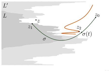
- [§4.1] Figures 15–17 illustrate the degree-3 family well, but the caption of Figure 5 (polygon splitting) could explicitly mark the valley σ and the two poles so that the mixed-cluster definition is immediately visible.
- A few typographical slips remain (e.g., occasional missing spaces after punctuation, and the arXiv identifier appears as 2607.06698). A final copy-edit pass would clean these.
Circularity Check
No significant circularity: regularity and structure theorems are transferred from independent parabolic/Sturmian analysis of the p-q dual IMCF clusters, not forced by definition or self-citation of the target claims.
full rationale
The paper defines ∞-harmonic functions independently (viscosity solutions of ∆_∞ u=0, or AMLE/comparison-with-cones) and constructs simple/mixed IMCF clusters independently (calibrated piecewise weak IMCF with outer-obstacle ridges/valleys). The bridge (process (1.15), Theorem 6.1) is a proved limit of classical p-q conjugates under the new C^{1} equicontinuity of p-harmonics (Theorem 5.1); support functions then satisfy the heat equation ∂_t h=∂_{ heta heta}h+h in the viscosity sense across cusps by direct comparison with sub/supersolutions (Theorem 7.1, Cases 1–2 and maximum principles of Remark 2.13), without presupposing C^{1,1/3}. Regularity of the resulting curves (C^{1,1/2} from nondegenerate roots of κ^{-1} via Sturmian theory) yields C^{0,1/3} normals and thus Theorem 1.1; isolation and blow-ups (Theorems 1.2–1.3) follow by the same IMCF-and-splitting analysis of sublevel sets of | abla u| (Sections 9–12) plus finite Fourier modes of the heat equation. Self-citations (e.g. [74] on obstacle IMCF) supply background tools whose statements do not contain the target C^{1,1/3} or isolation theorems, and the paper explicitly does not use the existence result of [74]. No fitted parameters, no self-definitional loop, and no uniqueness theorem that already encodes the claimed regularity. Residual risk is ordinary technical gap risk in a long geometric-PDE argument, not circularity.
Assumptions & free parameters
assumptions (6)
- standard math Equivalence of viscosity infinity-harmonicity, AMLE, comparison with cones, and C⁰_loc limits of p-harmonic functions (Jensen, Crandall–Evans–Gariepy, Bhattacharya–DiBenedetto–Manfredi).
- standard math Weak inverse mean curvature flow as local minimizers of J_w and the calibrated formulation div(ν)=|∇w| with |ν|≤1 (Huisken–Ilmanen).
- standard math Moser renormalization: (1−q)log v_q → weak IMCF as q→1 for positive q-harmonic v_q.
- standard math Sturmian root-counting for solutions of the 1D heat equation / ∂_t f = ∂_{θθ}f + f (Angenent).
- domain assumption Planar restriction: all main theorems are stated only in R²; duality and angle parametrization of curves are two-dimensional.
- ad hoc to paper Unit-calibrated mixed IMCF clusters produce C¹ infinity-harmonic functions via ∇u = e^{-w} ν^⊥ (Theorem 4.1).
invented entities (1)
-
Simple and mixed IMCF clusters (piecewise weak IMCF with outer-obstacle ridges and optional valleys/poles)
Cite this review
Pith. "Pith review of Infinity-harmonic functions and inverse mean curvature flow clusters." pith.science (2026). https://pith.science/paper/KRQU6GLZ
@misc{pith2026260706698,
  author       = {Pith},
  title        = {Pith review of: Infinity-harmonic functions and inverse mean curvature flow clusters},
  year         = {2026},
  howpublished = {\url{https://pith.science/paper/KRQU6GLZ}},
  note         = {Machine review of arXiv:2607.06698}
}
abstract
An $\infty$-harmonic function is a viscosity solution of $\nabla^2 u(\nabla u,\nabla u)=0$, or equivalently, an absolute minimizer of $\|\nabla u\|_{L^\infty}$. We prove a variety of new structural and regularity results in two dimensions, including: 1. $\infty$-harmonic functions in domains of $\mathbb{R}^2$ are $C^{1,1/3}$. 2. Critical points are isolated, and at each critical point, the solution has a unique quasiradial blow-up. 3. Entire solutions with polynomial growth have unique quasiradial blow-downs, and are determined by their Fourier modes at infinity. These results are consequences of a new theory relating $\infty$-harmonic functions to inverse mean curvature flow (IMCF) clusters -- which are piecewise weak solutions of IMCF with common obstacle-type boundary conditions on the interfaces (a simple example is an embedded family of cuspidal curves evolving by inverse curvature). This connection arises as the $p\to\infty$ limit of the classical duality between $p$-harmonic and $q$-harmonic functions in $\mathbb{R}^2$, where $\frac1p+\frac1q=1$.
Figures


Figures from the paper (38 more)








Reference graph
Works this paper leans on
-
[1]
Mass-type invariants in the presence of a cosmological constant
V. Agostiniani, S. Borghini, L. Mazzieri, Mass-type invariants in the presence of a cosmological constant, preprint (2026), arXiv:2603.01543
work page Pith review arXiv 2026
-
[2]
V. Agostiniani, C. Mantegazza, L. Mazzieri, F. Oronzio, Riemannian Penrose in- equality via nonlinear potential theory , Annali della Scuola Normale Superiore Classe di Scienze, page 27, 2025
work page 2025
- [3]
-
[4]
Angenent, The zero set of a solution of a parabolic equation , J
S. Angenent, The zero set of a solution of a parabolic equation , J. Reine. Angew. Math. 390 (1988), 79–96
work page 1988
-
[5]
Angenent, On the formation of singularities in the curve shortening flo w, J
S. Angenent, On the formation of singularities in the curve shortening flo w, J. Dif- ferential Geom. 33 (1991), no. 3, 601–633
work page 1991
-
[6]
S. Angenent, B. Fiedler, The dynamics of rotating waves in scalar reaction diffusion equations, Trans. Amer. Math. Soc. 307 (1988), no. 2, 545–568
work page 1988
- [7]
-
[8]
S. Armstrong, C. Smart, An easy proof of Jensen ’s theorem on the uniqueness of infinity harmonic functions , Calc. Var. Partial Differential Equations 37 (2010), no. 3-4, 381–384
work page 2010
Show all 75 references
-
[9]
Aronsson, Extension of functions satisfying Lipschitz conditions , Ark
G. Aronsson, Extension of functions satisfying Lipschitz conditions , Ark. Mat. 6, 1967, 551-561
1967
-
[10]
Aronsson, On the partial differential equation u2 xuxx + 2uxuyuxy +u2 yuyy = 0, Ark
G. Aronsson, On the partial differential equation u2 xuxx + 2uxuyuxy +u2 yuyy = 0, Ark. Mat. 7 (1968), 395–425
1968
-
[11]
Aronsson, On certain singular solutions of the partial differential eq uationu2 xuxx + 2uxuyuxy +u2 yuyy = 0, Manuscripta Math
G. Aronsson, On certain singular solutions of the partial differential eq uationu2 xuxx + 2uxuyuxy +u2 yuyy = 0, Manuscripta Math. 47 (1984), no. 1-3, 133–151
1984
-
[12]
Aronsson, Construction of singular solutions to the p-harmonic equation and its limit equation for p =∞ , Manuscripta Math
G. Aronsson, Construction of singular solutions to the p-harmonic equation and its limit equation for p =∞ , Manuscripta Math. 56 (1986), no. 2, 135–158
1986
-
[13]
Aronsson, M
G. Aronsson, M. Crandall, P. Juutinen, A tour of the theory of absolutely minimizing functions, Bull. Amer. Math. Soc. (N.S.) 41 (2004), no. 4, 439–505
2004
-
[14]
Aronsson, P
G. Aronsson, P. Lindqvist, On p-harmonic functions in the plane and their stream functions, J. Differential Equations 74 (1988), no. 1, 157–178
1988
-
[15]
Backus, An ∞ -Laplacian for differential forms, and calibrated laminati ons, preprint (2024), arXiv:2404.02215
A. Backus, An ∞ -Laplacian for differential forms, and calibrated laminati ons, preprint (2024), arXiv:2404.02215
2024 arXiv
-
[16]
Benatti, M
L. Benatti, M. Fogagnolo, L. Mazzieri, On the isoperimetric Riemannian Penrose inequality, Comm. Pure Appl. Math. 78 (2025), no. 5, 1042–1085
2025
-
[17]
Benatti, L
L. Benatti, L. Mari, M. Rigoli, A. Setti, K. Xu, Proper solutions of the 1/H -flow and the Green kernel of the p-Laplacian, preprint (2025), arXiv:2512.14591
2025
-
[18]
Benatti, A
L. Benatti, A. Pluda, M. Pozzetta, Fine properties of nonlinear potentials and a unified perspective on monotonicity formulas , preprint (2024), arXiv:2411.06462
2024
-
[19]
Bhattacharya, On the behaviour of ∞ -harmonic functions near isolated points , Nonlinear Analysis 58 (2004) 333–349
T. Bhattacharya, On the behaviour of ∞ -harmonic functions near isolated points , Nonlinear Analysis 58 (2004) 333–349
2004
-
[20]
Bhattacharya, A note on non-negative singular infinity-harmonic function s in the half-space, Rev
T. Bhattacharya, A note on non-negative singular infinity-harmonic function s in the half-space, Rev. Mat. Complut. 18 (2005), no. 2, 377–385
2005
-
[21]
Bhattacharya, E
T. Bhattacharya, E. DiBenedetto, J. Manfredi, Limits as p→∞ of ∆ pu = f and related extremal problems , Rend. Sem. Mat. Univ. Pol. Torino, Fascicolo Speciale 1989 Nonlinear PDE’s, 15-68. 148
1989
-
[22]
Brustad, The Infinity-Potential in the Square , preprint (2022), arxiv:2210.03447
K. Brustad, The Infinity-Potential in the Square , preprint (2022), arxiv:2210.03447
2022 arXiv
-
[23]
Brustad, Infinity-harmonic functions in the plane: Regularity by inj ectivity, preprint (2026), arXiv:2606.08257
K. Brustad, Infinity-harmonic functions in the plane: Regularity by inj ectivity, preprint (2026), arXiv:2606.08257
2026 arXiv
-
[24]
Brustad, E
K. Brustad, E. Lindgren, P. Lindqvist, The infinity-Laplacian in smooth convex do- mains and in a square , Math. Eng. 5 (2023), no. 4, Paper No. 080, 16 pp
2023
-
[25]
Castro, A
I. Castro, A. Lerma, Lagrangian homothetic solitons for the inverse mean curvat ure flow, Results Math. 71 (2017), no.3-4, 1109–1125
2017
-
[26]
Chow, D.-H
B. Chow, D.-H. Tsai, Geometric expansion of convex plane curves , J. Differential Geom. 44 (1996), no. 2, 312–330
1996
-
[27]
M. G. Crandall, A visit with the ∞ -Laplace equation, Calculus of Variations and Non- Linear Partial Differential Equations, Lecture Notes in Mathematic s 1927, Springer, Berlin, Heidelberg, pp. 75–122
1927
-
[28]
M. G. Crandall, L. C. Evans, R. F. Gariepy, Optimal Lipschitz extensions and the infinity laplacian , Calc. Var. Partial Differential Equations 13 (2001), no. 2, 123–1 39
2001
-
[29]
Crandall, H
M. Crandall, H. Ishii, P.-L. Lions, User’s guide to viscosity solutions of second order partial differential equations , Bull. Amer. Math. Soc. (N.S.) 27 (1992), no. 1, 1–67
1992
-
[30]
Daskalopoulos, K
G. Daskalopoulos, K. Uhlenbeck, Analytic properties of Stretch maps and geodesic laminations, preprint (2022), arXiv:2205.08250
2022 arXiv
-
[31]
Daskalopoulos, K
G. Daskalopoulos, K. Uhlenbeck, Transverse measures and best Lipschitz and least gradient maps , J. Differential Geom. 127 (2024), No. 3, 969-1018
2024
-
[32]
Daskalopoulos, K
G. Daskalopoulos, K. Uhlenbeck, Best Lipschitz maps and Earthquakes , preprint (2024), arXiv:2410.08296
2024 arXiv
-
[33]
H. Dong, F. Peng, Y. Zhang, Y. Zhou, Jacobian determinants for nonlinear gradient of planar∞ -harmonic functions and applications , J. Reine Angew. Math. 812 (2024), 59–98
2024
-
[34]
Drucker, S
D. Drucker, S. Williams, A note on Aronsson ’s equation, Rocky Mountain J. Math. 39 (2009), no. 6, 1859–1867
2009
-
[35]
Drugan, H
G. Drugan, H. Lee, G. Wheeler, Solitons for the inverse mean curvature flow , Pacific J. Math. 284 (2016), no. 2, 309–326
2016
-
[36]
L. C. Evans, O. Savin, C 1,α regularity for infinity harmonic functions in two dimen- sions, Calc. Var. Partial Differential Equations 32 (2008), no. 3, 325–3 47
2008
-
[37]
L. C. Evans, C. K. Smart, Everywhere differentiability of infinity harmonic function s, Calc. Var. Partial Differential Equations 42 (2011), no. 1-2, 289– 299
2011
-
[38]
L. C. Evans, C. K. Smart, Adjoint methods for the infinity Laplacian partial differ- ential equation , Arch. Ration. Mech. Anal. 201 (2011), no. 1, 87–113
2011
-
[39]
D. Gale, H. Nikaidˆ o, The Jacobian matrix and global univalence of mappings , Math. Ann. 159 (1965), 81–93
1965
-
[40]
Granlund, N
S. Granlund, N. Marola, Phragm´ en-Lindel¨ of theorem for infinity harmonic functions, Commun. Pure Appl. Anal. 14 (2015), no. 1, 127–132
2015
-
[41]
G´ orny, J
W. G´ orny, J. M. Maz´ on, Functions of least gradient , Monogr. Math., 110, Birkh¨ auser/Springer, Cham, 2024, xxviii+428 pp
2024
-
[42]
X. H. Han, Thurston norms, L2-norms, geodesic laminations, and Lipschitz maps , preprint (2023), arXiv:2310.18093
2023 arXiv
-
[43]
Huisken, T
G. Huisken, T. Ilmanen, The inverse mean curvature flow and the Riemannian Pen- rose inequality, J. Differential Geom. 59 (2001), no. 3, 353–437
2001
-
[44]
Ishii, On the equivalence of two notions of weak solutions, viscosi ty solutions and distribution solutions , Funkcial
H. Ishii, On the equivalence of two notions of weak solutions, viscosi ty solutions and distribution solutions , Funkcial. Ekvac. 38 (1995), no. 1, 101–120. 149
1995
-
[45]
Iwaniec, J
T. Iwaniec, J. Manfredi, Regularity of p-harmonic functions on the plane , Rev. Mat. Iberoamericana 5 (1989), no. 1-2, 1–19
1989
-
[46]
Jensen, Uniqueness of Lipschitz extensions: minimizing the sup nor m of the gra- dient, Arch
R. Jensen, Uniqueness of Lipschitz extensions: minimizing the sup nor m of the gra- dient, Arch. Rational Mech. Anal. 123 (1993), no. 1, 51-74
1993
-
[47]
H. Koch, Y. Zhang, Y. Zhou, An asymptotic sharp Sobolev regularity for planar infinity harmonic functions , J. Math. Pures Appl. (9) 132 (2019), 457–482
2019
-
[48]
Kotschwar, L
B. Kotschwar, L. Ni, Local gradient estimates of p-harmonic functions, 1/H -flow, and an entropy formula , Ann. Sci. ´Ec. Norm. Sup´ er. (4) 42 (2009), no. 1, 1–36
2009
-
[49]
D. A. Lee, Geometric Relativity, Graduate Studies in Mathematics, 201. American Mathematical Society, Providence, RI, 2019. xii+361 pp
2019
-
[50]
Lewis, Regularity of the derivatives of solutions to certain degen erate elliptic equa- tions, Indiana Univ
J. Lewis, Regularity of the derivatives of solutions to certain degen erate elliptic equa- tions, Indiana Univ. Math. J. 32 (1983), no. 6, 849–858
1983
-
[51]
G. M. Lieberman, Boundary regularity for solutions of degenerate elliptic e quations, Nonlinear Anal. 12 (1988), no. 11, 1203–1219
1988
-
[52]
Lindgren, P
E. Lindgren, P. Lindqvist, Infinity-harmonic potentials and their streamlines , Discrete Contin. Dyn. Syst. 39 (2019), no. 8, 4731–4746
2019
-
[53]
Lindgren, P
E. Lindgren, P. Lindqvist, The gradient flow of infinity-harmonic potentials , Adv. Math. 378 (2021), Paper No. 107526, 24 pp
2021
-
[54]
Lindqvist, Notes on the Infinity Laplace equation , SpringerBriefs Math, BCAM Basque Center for Applied Mathematics, Bilbao; Springer, [Cham], 20 16
P. Lindqvist, Notes on the Infinity Laplace equation , SpringerBriefs Math, BCAM Basque Center for Applied Mathematics, Bilbao; Springer, [Cham], 20 16. ix+68 pp
-
[55]
Lindqvist, J
P. Lindqvist, J. Manfredi, The Harnack inequality for ∞ -harmonic functions , Elec- tron. J. Differential Equations 1995, No. 04, approx. 5 pp
1995
-
[56]
Maggi, Sets of finite perimeter and geometric variational problems , an introduc- tion to geometric measure theory , Cambridge Stud
F. Maggi, Sets of finite perimeter and geometric variational problems , an introduc- tion to geometric measure theory , Cambridge Stud. Adv. Math., 135, Cambridge University Press, Cambridge, 2012. xx+454 pp
2012
-
[57]
Manfredi, p-harmonic functions in the plane , Proc
J. Manfredi, p-harmonic functions in the plane , Proc. Amer. Math. Soc. 103 (1988), no. 2, 473–479
1988
-
[58]
L. Mari, M. Rigoli, A. Setti, On the 1/H-flow by p-Laplace approximation: new estimates via fake distances under Ricci lower bounds , Amer. J. Math. 144 (2022), no. 3, 779–849
2022
-
[59]
J. M. Maz´ on, S. Segura de Le´ on, A non-homogeneous elliptic problem dealing with the level set formulation of the Inverse Mean Curvature Flow , J. Diff. Eq. 259 (2015), 2762–2806
2015
-
[60]
Moser, The inverse mean curvature flow and p-harmonic functions , J
R. Moser, The inverse mean curvature flow and p-harmonic functions , J. Eur. Math. Soc. (JEMS) 9 (2007), no.1, 77–83
2007
-
[61]
Moser, The inverse mean curvature flow as an obstacle problem , Indiana Univ
R. Moser, The inverse mean curvature flow as an obstacle problem , Indiana Univ. Math. J. 57 (2008), no. 5, 2235–2256
2008
-
[62]
Moser, The streamlines of∞ -harmonic functions obey the inverse mean curvature flow, Comm
R. Moser, The streamlines of∞ -harmonic functions obey the inverse mean curvature flow, Comm. Partial Differential Equations 47 (2022), no. 11, 2124–21 45
2022
-
[63]
Moser, A characterisation of ∞ -harmonic maps in terms of 1-currents , preprint (2026), arXiv:2606.10897
R. Moser, A characterisation of ∞ -harmonic maps in terms of 1-currents , preprint (2026), arXiv:2606.10897
2026 arXiv
-
[64]
S. B. Nadler Jr., Continuum theory. An introduction , Monogr. Textbooks Pure Appl. Math., 158, Marcel Dekker, Inc., New York, 1992. xiv+328 pp
1992
-
[65]
F. Peng, Y. Zhang, Y. Zhou, Regularity from p-harmonic potentials to ∞ -harmonic potentials in convex rings , Proc. Lond. Math. Soc. (3) 130 (2025), no. 6, Paper No. e70062, 54 pp. 150
2025
-
[66]
Peres, O
Y. Peres, O. Schramm, S. Sheffield, D. B. Wilson, Tug-of-war and the infinity Lapla- cian, J. Amer. Math. Soc. 22 (2009), no. 1, 167–210
2009
-
[67]
P´ olya, G
G. P´ olya, G. Szeg¨ o,Problems and Theorems in Analysis , Springer (Berlin), 1972
1972
-
[68]
Savin, C 1 regularity for infinity harmonic functions in two dimension s, Arch
O. Savin, C 1 regularity for infinity harmonic functions in two dimension s, Arch. Ration. Mech. Anal. 176 (2005), no. 3, 351–361
2005
-
[69]
Savin, C
O. Savin, C. Wang, Y. Yu, Asymptotic behavior of infinity harmonic functions near an isolated singularity , Int. Math. Res. Not. IMRN 2008 (6), Art. ID rnm163, 23 pp
2008
-
[70]
Simon, Lectures on geometric measure theory , Proc
L. Simon, Lectures on geometric measure theory , Proc. Centre Math. Anal. Austral. Nat. Univ., 3 Australian National University, Centre for Mathematic al Analysis, Canberra, 1983. vii+272 pp
1983
-
[71]
Urbas, Convex curves moving homothetically by negative powers of t heir curvature, Asian J
J. Urbas, Convex curves moving homothetically by negative powers of t heir curvature, Asian J. Math. 3 (1999), no. 3, 635–656
1999
-
[72]
Wang, An Introduction of Infinity Harmonic Functions , unpublished notes, 2008
C. Wang, An Introduction of Infinity Harmonic Functions , unpublished notes, 2008
2008
-
[73]
Xu, The weak inverse mean curvature flow: existence theories and applications, Ph.D
K. Xu, The weak inverse mean curvature flow: existence theories and applications, Ph.D. thesis, Duke University, 2025
2025
-
[74]
Xu, Inverse mean curvature flow with outer obstacle , preprint (2024), arxiv:2405.15181, to appear in Geom
K. Xu, Inverse mean curvature flow with outer obstacle , preprint (2024), arxiv:2405.15181, to appear in Geom. Topol
2024 arXiv
-
[75]
Zhang, Y
Y. Zhang, Y. Zhou, C 1-Regularity of planar ∞ -harmonic functions – revisited, Proc. Amer. Math. Soc. 148 (3), 2020, 1187–1193. Department of Mathematics, University of California, Berk eley. Email: kaixu@berkeley.edu 151
2020
Reviewed July 10, 2026 · model on record in the stance chip above.
Discussion (0). Continue with ORCID to comment.