REVIEW 2 major objections 7 minor 53 references
Multi-type Sensor Placement for PDE-based Bayesian Inverse Problems
T0 review · 2 major / 7 minor · reviewed 2026-07-10 · glm-5.2
Pith's one-line read Cheap sensors, pricey sensors: a greedy recipe for picking the best mix
desk verdict Multi-type sensor placement for PDE-based Bayesian inverse problems: knapsack-constrained greedy with BAE-based EIG lower bound for nonlinear problems read the letter →
The pith
A machine-rendered reading of the paper's core claim, the machinery that carries it, and where it could break.
The reading
What carries the argument
The argument rests on three pieces of machinery. First, the knapsack-constrained EIG formulation: each sensor has a cost c(v) and the design must satisfy c(S) ≤ B, replacing the usual cardinality constraint. Second, the stochastic cost-benefit greedy rule, which at each iteration samples T = c(V) log(1/ε)/B candidate sensors and selects the one maximizing the marginal-gain-to-cost ratio Δ(v|S)/c(v); the analysis chains an expected incremental-gain lemma (Lemma 3.2) through an induction to get E[f(S_k)] ≥ (1 − exp(−k(1−ε)/B)) f*. Third, the pure-BAE construction: the global linear operator F_O = Γ_{Fm} Γ_{mm}^{-1} (the cross-covariance of the forward output and the parameter, times the prior-
What would settle it
A nonlinear PDE-based inverse problem where the BAE lower-bound gap Ψ_MT − Ψ^O_MT varies substantially across designs, causing the surrogate-optimal design to be far from the true-EIG-optimal design. Such a counterexample would show that the lower-bound property alone is insufficient to justify the surrogate as an optimization objective.
Extended reading notes
Core claim
The paper establishes that for nonlinear Bayesian inverse problems with Gaussian priors, the expected information gain computed from the pure-BAE global linear model (an error-corrected, data-driven linear surrogate requiring no Jacobian evaluations) is a provable lower bound on the exact EIG. This transforms the surrogate from a heuristic proxy into a principled objective for knapsack-constrained sensor placement. A complementary contribution is the stochastic cost-benefit greedy algorithm, which provides an expected approximation ratio for monotone submodular maximization under knapsack constraints while requiring only O(c(V) log(1/ε)) marginal-gain evaluations.
Load-bearing premise
The effectiveness of the pure-BAE EIG as a proxy for the exact EIG in nonlinear problems depends on the gap between the true EIG and the surrogate being roughly uniform across candidate designs. The paper proves the gap is non-negative but provides no theoretical guarantee of its uniformity; the claim rests on a single numerical example.
Editorial extensions
If this is right
- The stochastic cost-benefit greedy algorithm and its approximation guarantee apply to any monotone submodular maximization problem under a knapsack constraint, not just sensor placement for inverse problems.
- The lower-bound result means practitioners can perform nonlinear OED without adjoint solves or Jacobian computations, using only input-output pairs from the forward model—a significant simplification for black-box or legacy simulation codes.
- The gap formula Ψ_MT − Ψ^O_MT = E_{π_d}[D_KL(π_{m|d} ∥ π^O_{m|d})] provides a concrete diagnostic: if the gap is roughly constant across candidate designs, the surrogate preserves the ranking of designs and the approach is trustworthy; if it varies, the surrogate may mislead.
- The connection to Stein's lemma (Theorem 4.2) suggests that the prior-expected Jacobian could serve as a natural linearization point in other contexts, such as uncertainty quantification or reduced-order modeling, beyond experimental design.
Reading between the lines
- If the BAE lower bound gap varies significantly across designs in some problem class, the method could systematically prefer designs where the linear surrogate is poor rather than where the true information gain is high. The paper's single nonlinear numerical example is insufficient to rule this out for general nonlinear PDE problems with strong non-Gaussian posteriors.
- The non-submodularity of the pure-BAE EIG (due to the non-diagonal total-error covariance) means the greedy algorithm's empirical success in the nonlinear case is not covered by the linear-case theory. A problem class where greedy fails for non-submodular objectives would expose the limits of the approach.
- Extending the lower-bound argument to non-Gaussian priors introduces a design-independent correction term, which the paper notes but does not develop; whether this correction term is truly design-independent for structured non-Gaussian priors (e.g., mixture priors) is an open question.
Editorial analysis
A structured set of objections, weighed in public.
Referee Report
Summary. This paper addresses optimal placement of multi-type sensors (different costs, accuracies, and observation types) for Bayesian inverse problems governed by PDEs. For linear Gaussian inverse problems with uncorrelated noise, the EIG is monotone submodular, and the authors propose a stochastic cost-benefit greedy algorithm (Algorithm 3.1) with an approximation guarantee under knapsack constraints (Theorem 3.3). For nonlinear inverse problems, the authors develop a non-intrusive framework based on the Bayesian approximation error (BAE) approach, constructing a pure-BAE global linear model F_O = Γ_{Fm} Γ_{mm}^{-1}. They prove (Theorem 4.2) that this operator equals the prior expectation of the Jacobian of the parameter-to-observable map, and (Theorem 4.5) that the corresponding pure-BAE EIG is a lower bound on the exact EIG. The methods are demonstrated on a linear source inversion problem and a nonlinear porous-medium flow problem.
Significance. The paper makes two distinct theoretical contributions. First, the stochastic cost-benefit greedy algorithm and its approximation guarantee (Theorem 3.3, Corollary 3.4) extend stochastic greedy methods to the knapsack-constrained submodular setting in a principled way; this is of independent interest beyond sensor placement. Second, the lower bound result (Theorem 4.5) — that the pure-BAE EIG lower-bounds the exact EIG for nonlinear problems with Gaussian priors — provides a rigorous justification for using a computationally cheap surrogate in the OED loop. The connection to the expected Jacobian (Theorem 4.2, a multidimensional Stein's lemma) is a nice interpretive result. The non-intrusive nature of the BAE approach (no adjoint solves needed) is a practical strength. The numerical experiments are reasonably comprehensive, including comparison against NMC-based greedy designs.
major comments (2)
- Section 4.3, paragraph after Theorem 4.5: The practical justification for using Ψ^O_MT as the OED objective for nonlinear problems rests on the assumption that the gap Ψ_MT − Ψ^O_MT = E_{π_d}[D_KL(π_{m|d} ∥ π^O_{m|d})] does not vary significantly across designs S. The authors acknowledge this is unproven and support it only with the single numerical example in Section 5.2. This is the load-bearing assumption for the practical (nonlinear) claim. While the lower bound theorem itself is correct and cleanly proven, the paper would benefit from either (a) a more detailed discussion of conditions under which the gap is approximately design-independent, or (b) at minimum, a second nonlinear test problem with a different nonlinearity structure to strengthen the empirical evidence. As it stands, the leap from valid lower bound to effective surrogate is bridged by one example.
- Algorithm 3.1, line 4 vs. Lemma 3.2: The algorithm states that R is a 'random subset' of the remaining feasible sensors, which suggests sampling without replacement. However, the proof of Lemma 3.2 (and Lemma A.2) uses a binomial distribution argument that assumes sampling with replacement. This discrepancy should be clarified: is R sampled with or without replacement? If without replacement, the binomial argument in Lemma A.2 needs modification. If with replacement, the algorithm description should say so explicitly, and the practical implications (possibly selecting the same sensor multiple times in the inner loop) should be addressed.
minor comments (7)
- Section 3.3, Eq. (3.15): The approximation ratio depends on C̄ = max_v c(v), which can be arbitrarily large relative to B, making the bound vacuous in some settings. A brief remark on when this bound is non-trivial (e.g., when costs are within a bounded range of each other) would help the reader calibrate expectations.
- Section 5.2.1: The packing constraint (at most one sensor type per location) is introduced informally. It would help to state precisely how this modifies the optimization problem and why the greedy algorithms still apply (or are heuristically adapted).
- Section 5.2.2: The choice N=5000 samples for BAE statistics is stated as 'sufficiently stable empirically' but no convergence study or sensitivity analysis is provided. A brief remark on how the design quality depends on N would strengthen the practical guidance.
- Section 4.4, last paragraph: The note that lazy evaluations are 'neither justified nor recommended' without submodularity is important but buried. Consider highlighting this more prominently, as practitioners may be tempted to use lazy evaluations based on the linear-case discussion.
- Figure 7 (right): The histogram axis labels and binning are somewhat hard to read. Consider adding tick marks or a summary statistic (e.g., median gap) to aid interpretation.
- Section 2.1: The notation π = N(x̄, Γ_xx) is introduced but the shorthand is used inconsistently; sometimes the full N(·,·) notation is used. Minor consistency fix.
- The reference list includes several 2025–2026 entries (e.g., [3], [5], [38], [41]) that appear to be preprints or forthcoming. Ensure final publication details are updated upon acceptance.
Circularity Check
No significant circularity; derivations are self-contained from standard mathematical tools
full rationale
The paper's three main theoretical results are derived from first principles using standard mathematical machinery, with no circular or self-definitional structure. (1) Theorem 4.5 (lower bound Ψ_MT ≥ Ψ^O_MT) is proven via the KL-divergence chain rule and the moment-matching property of Lemma 4.3, which itself follows by direct calculation from the definitions in (4.6). The gap is shown to equal E_{π_d}[D_KL(π_{m|d} ∥ π^O_{m|d})] ≥ 0, which is non-negative by the non-negativity of KL divergence — not by construction or tautology. (2) Theorem 4.2 (pure-BAE operator = E[J(m)]) is a multidimensional Stein's lemma derivation, proven by integration by parts (Lemma 4.1 / divergence theorem). (3) Theorem 3.3 (stochastic greedy approximation ratio) follows from standard submodular optimization arguments (Lemma 3.2 on expected incremental gain, induction). The self-citations ([5, 26, 37]) provide building blocks (e.g., the BAE framework, invariance of the error-aware likelihood to the choice of linearization) but are not load-bearing in a circular way: Theorem 4.5's proof does not depend on any unverified claim from the authors' prior work. The practical concern — that the gap between the lower bound and the exact EIG may vary across designs, potentially affecting the surrogate's ranking — is a correctness/effectiveness concern, not a circularity issue, and is honestly acknowledged by the authors (paragraph after Theorem 4.5). No 'prediction' reduces to a fitted input, no uniqueness theorem is invoked to forbid alternatives, and no ansatz is smuggled in via self-citation. The derivations are self-contained against external mathematical standards.
Assumptions & free parameters
free parameters (5)
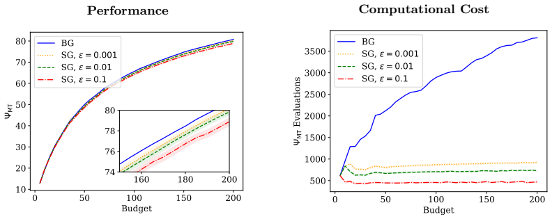
- Approximation parameter ε =
0.001, 0.01, 0.1
- Budget B =
30 (linear), 15 (nonlinear)
- Sensor costs c(v) =
1, 2.8, 5 (linear); 1, 1.5 (nonlinear)
- Prior parameters γ, δ =
γ=0.252, δ=0.7 (linear); γ=0.1, δ=0.5 (nonlinear)
- Number of BAE samples N =
5000
assumptions (4)
- domain assumption Gaussian prior and additive Gaussian noise with uncorrelated measurement errors
- ad hoc to paper EIG gap uniformity across designs
- domain assumption Finite differential entropy of π_{d,m}
- domain assumption F is differentiable and bounded (or satisfies Remark 4.1)
Cite this review
Pith. "Pith review of Multi-type Sensor Placement for PDE-based Bayesian Inverse Problems." pith.science (2026). https://pith.science/paper/S47RKZSR
@misc{pith2026260708074,
  author       = {Pith},
  title        = {Pith review of: Multi-type Sensor Placement for PDE-based Bayesian Inverse Problems},
  year         = {2026},
  howpublished = {\url{https://pith.science/paper/S47RKZSR}},
  note         = {Machine review of arXiv:2607.08074}
}
read the original abstract
We address optimal placement of multi-type sensors for Bayesian inverse problems governed by partial differential equations (PDEs). The proposed framework allows for sensors with different accuracies and observation types. We formulate the optimal experimental design (OED) problem as a knapsack-constrained binary optimization problem for maximizing expected information gain (EIG). To approximately solve the resulting optimization problems, we propose a stochastic cost-benefit greedy algorithm, which admits theoretical guarantees for monotone submodular set functions. Specifically, these guarantees apply in the case of linear Gaussian inverse problems with uncorrelated measurement errors, where the EIG admits a convenient closed-form expression. For nonlinear inverse problems, we develop a non-intrusive approach that uses the Bayesian approximation error framework to define an observation model with an error-corrected global linear model. We show that the corresponding approximate EIG is a lower bound for the exact EIG and thus provides a principled surrogate objective for the OED problem. The effectiveness of the proposed methods is demonstrated in two model inverse problems governed by PDEs.
Figures


Figures from the paper (4 more)


Reference graph
Works this paper leans on
-
[34]
B. Mirzasoleiman, A. Badanidiyuru, A. Karbasi, J. Vondr´ ak, and A. Krause. Lazier than lazy greedy. In Proceedings of the AAAI Conference on Artificial Intelligence, volume 29, pages 1867–1873, 2015
work page 2015
-
[1]
C. Aarset. Global optimality conditions for sensor placement, with extensions to binary low-rank A- optimal designs.Inverse Problems, 41(6):065013, 2025
work page 2025
-
[2]
A. Alexanderian. Optimal experimental design for infinite-dimensional Bayesian inverse problems gov- erned by PDEs: A review.Inverse Problems, 37(4):043001, 2021
work page 2021
-
[3]
Alexanderian.Computational Inverse Problems Governed by PDEs
A. Alexanderian.Computational Inverse Problems Governed by PDEs. SIAM, 2026
work page 2026
-
[4]
A. Alexanderian, P. J. Gloor, and O. Ghattas. On Bayesian A-and D-optimal experimental designs in infinite dimensions.Bayesian Anal., 11(3):671–695, 2016
work page 2016
-
[5]
Submodularity of the expected information gain in infinite-dimensional linear inverse problems
A. Alexanderian and S. Maio. Submodularity of the expected information gain in infinite-dimensional linear inverse problems.arXiv preprint arXiv:2602.09285, 2026
work page Pith review arXiv 2026
-
[6]
A. Alexanderian, R. Nicholson, and N. Petra. Optimal design of large-scale nonlinear Bayesian inverse problems under model uncertainty.Inverse Problems, 40(9):095001, 2024
work page 2024
-
[7]
A. Alexanderian and A. K. Saibaba. Efficient D-optimal design of experiments for infinite-dimensional Bayesian linear inverse problems.SIAM J. Sci. Comput., 40(5):A2956–A2985, 2018
work page 2018
Show all 53 references
-
[8]
Badanidiyuru and J
A. Badanidiyuru and J. Vondr´ ak. Fast algorithms for maximizing submodular functions. InProceedings of the twenty-fifth annual ACM-SIAM symposium on Discrete algorithms, pages 1497–1514, 2014
2014
-
[9]
I. A. Baratta, J. P. Dean, J. S. Dokken, M. Habera, J. S. Hale, C. N. Richardson, M. E. Rognes, M. W. Scroggs, N. Sime, and G. N. Wells. DOLFINx: The next generation FEniCS problem solving environment. Preprint, 2023
2023
-
[10]
Brezzi, J
F. Brezzi, J. Douglas Jr, and L. D. Marini. Two families of mixed finite elements for second order elliptic problems.Numer. Math., 47(2):217–235, 1985
1985
-
[11]
Clark, S
E. Clark, S. L. Brunton, and J. N. Kutz. Multi-fidelity sensor selection: Greedy algorithms to place cheap and expensive sensors with cost constraints.IEEE Sens. J., 21(1):600–611, 2020
2020
-
[12]
T. M. Cover.Elements of Information Theory. John Wiley & Sons, 1999
1999
-
[13]
T. Cui, K. Koval, R. Herzog, and R. Scheichl. Subspace accelerated measure transport methods for fast and scalable sequential experimental design, with application to photoacoustic imaging.arXiv preprint arXiv:2502.20086, 2025
2025 arXiv
-
[14]
Duong, T
D.-L. Duong, T. Helin, and J. R. Rojo-Garcia. Stability estimates for the expected utility in Bayesian optimal experimental design.Inverse Problems, 39(12):125008, 2023
2023
-
[15]
H. C. Elman, D. J. Silvester, and A. J. Wathen.Finite Elements and Fast Iterative Solvers: With Applications in Incompressible Fluid Dynamics. Oxford university press, 2014
2014
-
[16]
L. C. Evans.Partial Differential Equations, volume 19. American mathematical society, 2022
2022
-
[17]
L. G. Everett.Monitoring Groundwater Quality: Methods and Costs. US Environmental Protection Agency, Office of Research and Development, 1976
1976
-
[18]
Go and P
J. Go and P. Chen. Accurate, scalable, and efficient Bayesian optimal experimental design with derivative- informed neural operators.Comput. Methods Appl. Mech. Engrg., 438:117845, 2025
2025
-
[19]
Haber, L
E. Haber, L. Horesh, and L. Tenorio. Numerical methods for experimental design of large-scale linear ill-posed inverse problems.Inverse Problems, 24(5):055012, 2008
2008
-
[20]
Herman, A
E. Herman, A. Alexanderian, and A. K. Saibaba. Randomization and reweightedℓ 1-minimization for A-optimal design of linear inverse problems.SIAM J. Sci. Comput., 42(3):A1714–A1740, 2020
2020
-
[21]
X. Huan, J. Jagalur, and Y. Marzouk. Optimal experimental design: Formulations and computations. Acta Numer., 33:715–840, 2024
2024
-
[22]
Huan and Y
X. Huan and Y. M. Marzouk. Simulation-based optimal Bayesian experimental design for nonlinear systems.J. Comput. Phys., 232(1):288–317, 2013
2013
-
[23]
Huttunen and J
J. Huttunen and J. Kaipio. Approximation error analysis in nonlinear state estimation with an application to state-space identification.Inverse Problems, 23(5):2141, 2007
2007
-
[24]
Kaipio and V
J. Kaipio and V. Kolehmainen. Approximate marginalization over modelling errors and uncertainties in inverse problems. InBayesian Theory and Applications. Oxford University Press, 01 2013
2013
-
[25]
Kaipio and E
J. Kaipio and E. Somersalo. Statistical inverse problems: discretization, model reduction and inverse crimes.Journal of computational and applied mathematics, 198(2):493–504, 2007
2007
-
[26]
Koval and R
K. Koval and R. Nicholson. Non-intrusive optimal experimental design for large-scale nonlinear Bayesian inverse problems using a Bayesian approximation error approach.J. Sci. Comput., 104(3):98, 2025
2025
-
[27]
Krause and D
A. Krause and D. Golovin. Submodular function maximization. In L. Bordeaux, Y. Hamadi, and P. Kohli, 28 editors,Tractability: Practical Approaches to Hard Problems, pages 71–104. Cambridge University Press, 2014
2014
-
[28]
Krause and C
A. Krause and C. Guestrin. A note on the budgeted maximization of submodular functions. Technical report, Carnegie Mellon University, 2005
2005
-
[29]
Krause, A
A. Krause, A. Singh, and C. Guestrin. Near-optimal sensor placements in Gaussian processes: Theory, efficient algorithms and empirical studies.J. Mach. Learn. Res., 9(2), 2008
2008
-
[30]
Kulik, H
A. Kulik, H. Shachnai, and T. Tamir. Maximizing submodular set functions subject to multiple linear constraints. InProceedings of the twentieth annual ACM-SIAM symposium on Discrete algorithms, pages 545–554, 2009
2009
-
[31]
Logg, K.-A
A. Logg, K.-A. Mardal, and G. Wells.Automated Solution of Differential Equations by the Finite Element Method: The FEniCS Book, volume 84. Springer Science & Business Media, 2012
2012
-
[32]
S. Lunz, A. Hauptmann, T. Tarvainen, C.-B. Schonlieb, and S. Arridge. On learned operator correction in inverse problems.SIAM J. Imaging Sci., 14(1):92–127, 2021
2021
-
[33]
M. Minoux. Accelerated greedy algorithms for maximizing submodular set functions. In J. Stoer, editor, Optimization Techniques II, volume 7 ofLecture Notes in Control and Information Sciences, pages 234–243. Springer, Berlin, Heidelberg, 1978
1978
-
[35]
K. P. Murphy.Probabilistic machine learning: Advanced topics. MIT press, 2023
2023
-
[36]
G. L. Nemhauser, L. A. Wolsey, and M. L. Fisher. An analysis of approximations for maximizing sub- modular set functions—I.Math. Programming, 14(1):265–294, 1978
1978
-
[37]
Nicholson, N
R. Nicholson, N. Petra, U. Villa, and J. P. Kaipio. On global normal linear approximations for nonlinear Bayesian inverse problems.Inverse Problems, 39(5):054001, 2023
2023
-
[38]
Nicholson, R
R. Nicholson, R. Vuchkov, U. Villa, and N. Petra. Taylor approximation variance reduction for ap- proximation errors in PDE-constrained Bayesian inverse problems.Inverse Problems, 42(4):045020, 2026
2026
-
[39]
V. V. Petrov. On lower bounds for tail probabilities.J. Statist. Plann. Inference, 137(8):2703–2705, 2007
2007
-
[40]
Poole, S
B. Poole, S. Ozair, A. Van Den Oord, A. Alemi, and G. Tucker. On variational bounds of mutual information. InInternational conference on machine learning, pages 5171–5180. PMLR, 2019
2019
-
[41]
Ramon, G
G. Ramon, G. Sarnoski, V. Tumuluri, H. D´ ıaz, and A. K. Saibaba. Multifidelity sensor placement in Bayesian state estimation problems, 2026. arXiv:2602.07269
2026
-
[42]
Roininen, J
L. Roininen, J. M. Huttunen, and S. Lasanen. Whittle-Mat´ ern priors for Bayesian statistical inversion with applications in electrical impedance tomography.Inverse Probl. Imaging, 8(2), 2014
2014
-
[43]
K. J. Ryan. Estimating expected information gains for experimental designs with application to the random fatigue-limit model.J. Comput. Graph. Statist., 12(3):585–603, 2003
2003
-
[44]
Shamaiah, S
M. Shamaiah, S. Banerjee, and H. Vikalo. Greedy sensor selection: Leveraging submodularity. In49th IEEE Conference on Decision and Control (CDC), pages 2572–2577, Atlanta, GA, USA, 2010
2010
-
[45]
C. M. Stein. Estimation of the mean of a multivariate normal distribution.The Annals of Statistics, 9(6):1135–1151, 1981
1981
-
[46]
A. Stuart. Inverse problems: a Bayesian perspective.Acta Numer., 19:451–559, 2010
2010
-
[47]
Sviridenko
M. Sviridenko. A note on maximizing a submodular set function subject to a knapsack constraint.Oper. Res. Lett., 32(1):41–43, Jan. 2004
2004
-
[48]
Thibaut, N
R. Thibaut, N. Compaire, N. Lesparre, M. Ramgraber, E. Laloy, and T. Hermans. Comparing well and geophysical data for temperature monitoring within a Bayesian experimental design framework. Water Resour. Res., 58(11):e2022WR033045, 2022
2022
-
[49]
Uci´ nski.Optimal Measurement Methods for Distributed Parameter System Identification
D. Uci´ nski.Optimal Measurement Methods for Distributed Parameter System Identification. CRC Press, Boca Raton, 2005
2005
-
[50]
Ambient ground water quality monitoring cost analy- sis
United States Environmental Protection Agency. Ambient ground water quality monitoring cost analy- sis. Technical Report EPA 816-R-97-013, Office of Water, United States Environmental Protection Agency, Washington, DC, Oct. 1997
1997
-
[51]
Villa, N
U. Villa, N. Petra, and O. Ghattas. hippylib: An extensible software framework for large-scale inverse problems.J. Open Source Softw., 3(30), 2018
2018
-
[52]
K. Wu, P. Chen, and O. Ghattas. A fast and scalable computational framework for large-scale high- dimensional Bayesian optimal experimental design.SIAM/ASA J. Uncertain. Quantif., 11(1):235– 29 261, 2023
2023
-
[53]
K. Wu, T. O’Leary-Roseberry, P. Chen, and O. Ghattas. Large-scale Bayesian optimal experimental design with derivative-informed projected neural network.J. Sci. Comput., 95(1), 2023. Appendix A. Stochastic Cost-Benefit Greedy Auxiliary Results. The following results are used i...
2023
Reviewed July 10, 2026 · model on record in the stance chip above.
Discussion (0). Continue with ORCID to comment.