REVIEW 4 minor 58 references
An Explicit Link between Extreme Value Theory and Compositional Data Analysis
T0 review · 0 major / 4 minor · reviewed 2026-07-13 · grok-4.5
Pith's one-line read Extreme-value and compositional covariances are the same matrices, linked by three maps, so methods transfer both ways.
desk verdict Clean algebraic unification of Hüsler–Reiss and Aitchison covariance languages that immediately yields usable transfers both ways. read the letter →
The pith
A machine-rendered reading of the paper's core claim, the machinery that carries it, and where it could break.
The reading
What carries the argument
The commutative diagram of Proposition 4.1: three elementary maps—the variogram map γ, the covariance projections π_{1v^⊥} along the all-ones vector, and the Moore–Penrose inverse—that organise all the rank-deficient covariance and precision objects appearing in both fields.
What would settle it
Find a Hüsler–Reiss dataset and a compositional dataset whose estimated variation-array / extremal-variogram matrices cannot be mapped into each other by the three operations of the diagram, or show that an intrinsic logistic-normal graph recovered by the adapted algorithm fails to recover the true sparsity pattern of the centred precision on synthetic data generated from Definition 5.1.
Extended reading notes
Core claim
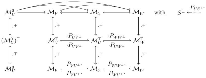
The extremal variogram, the family of extremal-function covariance and precision matrices of a Hüsler–Reiss model, and the compositional variation array together with its centred and additive log-ratio covariances are precisely the matrices of Proposition 4.1: they are related by the three maps γ (variogram), π_{1v^⊥} (covariance projection along the all-ones direction) and the Moore–Penrose inverse, so every representation in one field is algebraically identical to a representation in the other.
Load-bearing premise
Every component must be fully present (no asymptotic independence in extremes, no zeros on the simplex), so that the relative structure lives on a single hyperplane complementary to the all-ones vector.
Editorial extensions
If this is right
- Sparse precision patterns learned for Hüsler–Reiss extremes become intrinsic logistic-normal graphical models for compositional data, estimated by the majority-vote algorithm cglearn.
- Log-ratio analysis, weighted biplots, amalgamation clustering and stepwise log-ratio selection become off-the-shelf exploratory tools for extremal functions and extremal variograms.
- A single soft-threshold weighted estimator of the extremal variogram can replace hard thresholding by re-using the row-weighting idea of weighted log-ratio analysis.
- Any future algorithm that manipulates one of the matrices in the diagram automatically yields a corresponding algorithm in the other field by applying the three maps.
Reading between the lines
- Once zeros and asymptotic independence are handled by the subface or replacement methods already sketched in the outlook, the same diagram would organise mixture models across disconnected components, giving a common language for both fields’ sparse substructures.
- The two-dimensional kernel case (all-ones plus a decay-rate vector) suggested by linear compositional processes would immediately supply a time-inhomogeneous analogue of the extremal variogram that has not yet been used in extremes.
- Because the algebraic correspondence is basis-free, software libraries for one field can be wrapped rather than rewritten, lowering the barrier to cross-domain applications in geochemistry, hydrology and ecology.
Editorial analysis
A structured set of objections, weighed in public.
Referee Report
Summary. The paper establishes an algebraic identification between the covariance structures of Hüsler–Reiss multivariate extremes and those of Aitchison compositional data analysis. Both families are shown to sit inside the same commutative diagram (Proposition 4.1, Figure 5) generated by three maps: the variogram map γ, the family of covariance projections π_{1v^⊥} along the all-ones vector, and the Moore–Penrose inverse. Corollaries 4.2 and 4.6 specialise the diagram to the extremal variogram / extremal-function covariances / singular precision matrices of a Hüsler–Reiss model and to the compositional variation array / CLR / ALR covariances of a composition. The identification is then used to transfer methods in both directions: an intrinsic logistic-normal graphical model for compositions (Definition 5.1, Algorithm 1 cglearn) is obtained from Hüsler–Reiss graphical models, while log-ratio analysis, weighted LRA, amalgamation clustering and stepwise log-ratio selection are applied to extremal functions (Danube data). Full proofs of the projection and pseudoinverse identities appear in Appendices A–C.
Significance. If the algebraic identification holds, the paper supplies a clean, parameter-free dictionary that lets practitioners move covariance estimators, graphical models and dimension-reduction tools between two mature literatures that have previously only been linked informally. The central diagram is pure linear algebra (verified by direct Moore–Penrose and kernel–image arguments), so the transfer is not an analogy but an exact specialisation. Concrete deliverables include a new class of intrinsic logistic-normal graphical models for compositions, the cglearn algorithm, and the first systematic application of weighted LRA and amalgamation clustering to multivariate extremes. The scope restriction to full asymptotic dependence / strictly positive compositions is stated explicitly (§6.1) and does not undermine the diagram itself. The work therefore constitutes a genuine methodological bridge rather than a re-packaging of existing results.
minor comments (4)
- In §5.1.3 the comparison of cglearn with CCLasso on the gemas data is purely descriptive (shared-edge ratios). A short simulation under the intrinsic logistic-normal model that reports edge-recovery rates for both methods would make the relative performance clearer.
- Figure 11 shows a modest MSE gain for the weighted variogram estimator, but the simulation design (n=1000, d=10, single Γ) is narrow. A brief remark on sensitivity to the radial-weight choice would help readers judge robustness.
- Notation for the singular precision Θ₁ is introduced in (2.6) and reused for compositions; a one-sentence reminder in §4.3 that the same symbol now denotes the CLR precision would reduce momentary confusion for readers coming from only one of the two fields.
- The reference list already covers the main EVT and CoDA sources; adding the recent geometric modelling paper of Kakampakou & Wadsworth (2025) cited in the introduction would complete the “prior parallels” paragraph.
Circularity Check
No significant circularity: the claimed link is an algebraic identification verified by direct projection and Moore–Penrose identities, not a prediction forced by its inputs.
full rationale
The paper’s central claim is that the extremal variogram / compositional variation array, the family of projected covariances Σ_v (including CLR and ALR forms), and their Moore–Penrose precisions Θ_v are exactly the objects related by the three maps of Proposition 4.1 (variogram map γ, covariance projections π_{1v^⊥}, and pseudoinverse). Section 3 defines oblique projections and covariance projections for general complementary subspaces; Lemma 3.4 and Proposition 4.1 then verify the required kernel–image and Moore–Penrose relations by direct calculation (Appendix C). Corollaries 4.2 and 4.6 simply specialise those identities to Hüsler–Reiss extremal functions and to log-ratio covariances of compositions; no parameter is fitted to produce the claimed equivalence. Later methodological transfers (intrinsic logistic-normal graphical models via cglearn, weighted LRA / amalgamation applied to extremal functions) inherit the same non-circular character: they reuse the algebraic correspondence rather than re-deriving it from data. Self-citations to the authors’ prior EVT work supply background definitions of extremal functions and Hüsler–Reiss graphical models, but the uniqueness of the diagram and the transfer constructions are proved inside the paper and do not rest on an unverified self-citation chain. The full-asymptotic-dependence / no-zeros restriction is an explicit scope assumption (§6.1), not a circular step. Score 0 is therefore the honest finding.
Assumptions & free parameters
free parameters (3)
- graphical-lasso / neighbourhood-selection penalty λ
- threshold probability p for extremal sample
- observation weights r_k in weighted variogram
assumptions (3)
- standard math Oblique projectors along complementary subspaces are well-defined and satisfy the product and inverse relations of Lemma 3.2
- domain assumption Hüsler–Reiss extremal functions are Gaussian with covariances related by the stated projections (Corollary 4.2)
- domain assumption Compositional data are strictly positive so that all log-ratios exist (and, dually, full asymptotic dependence so that no component is −∞)
invented entities (1)
-
intrinsic logistic-normal graphical model
Cite this review
Pith. "Pith review of An Explicit Link between Extreme Value Theory and Compositional Data Analysis." pith.science (2026). https://pith.science/paper/K7YM5SM2
@misc{pith2026260709567,
  author       = {Pith},
  title        = {Pith review of: An Explicit Link between Extreme Value Theory and Compositional Data Analysis},
  year         = {2026},
  howpublished = {\url{https://pith.science/paper/K7YM5SM2}},
  note         = {Machine review of arXiv:2607.09567}
}
read the original abstract
Extreme value theory and compositional data analysis both study settings where relative information plays a central role. In multivariate extreme value theory, threshold exceedance limits satisfy homogeneity properties that separate the radial size of an extreme event from its relative profile. In compositional data analysis, positive vectors are analysed up to multiplicative scale, and inference is based on ratios or log-ratios between components. Consequently, both fields have developed several covariance and dependence representations of the underlying relative structure. In the H\"usler-Reiss model for extremes, these include variogram, covariance, and precision parametrizations. In compositional data analysis, analogous representations arise from pairwise log-ratios, centred log-ratios, and additive log-ratios. We establish an explicit link between the two fields that relates these different representations by a small set of simple transformations, including oblique projections, H\"usler-Reiss inverses, and the variogram map. From a methodological perspective, leveraging this algebraic connection enables the transfer of statistical approaches from one field to the other. For instance, we introduce intrinsic logistic-normal graphical models for compositional data, which are based on H\"usler-Reiss graphical models for extremes. Conversely, we explore how dimensionality reduction methods from compositional data analysis can be applied to the analysis of multivariate extremes.
Figures


Figures from the paper (11 more)



Reference graph
Works this paper leans on
-
[1]
Afriat, S. N. (1957). Orthogonal and oblique projectors and the characteristics of pairs of vector spaces. Mathematical Proceedings of the Cambridge Philosophical Society , 53:800 -- 816
1957
-
[2]
Aitchison, J. (1983). Principal component analysis of compositional data. Biometrika , 70(1):57--65
1983
-
[3]
Aitchison, J. (1986). The Statistical Analysis of Compositional Data . Springer Netherlands, Dordrecht. OCLC: 858944307
1986
-
[4]
C., and Engelke, S
Asadi, P., Davison, A. C., and Engelke, S. (2015). Extremes on river networks. Ann. Appl. Statist. , 9(4):2023--2050
2015
-
[5]
L., and Segers, J
Beirlant, J., Goegebeur, Y., Teugels, J. L., and Segers, J. (2004). The Secura Belgian Re Data , chapter 6.2. Wiley Series in Probability and Statistics. John Wiley & Sons, Ltd, Chichester. Section 6.2 in Chapter 6, Case Studies
2004
-
[6]
Billheimer, D., Guttorp, P., and Fagan, W. F. (2001). Statistical interpretation of species composition. Journal of the American Statistical Association , 96(456):1205--1214
2001
-
[7]
Chiapino, M., Sabourin, A., and Segers, J. (2019). Identifying groups of variables with the potential of being large simultaneously. Extremes , 22
2019
-
[8]
Coles, S., Heffernan, J., and Tawn, J. (1999). Dependence measures for extreme value analyses. Extremes , 2:339--365
1999
Show all 58 references
-
[9]
Coles, S. G. and Tawn, J. A. (1991). Modelling extreme multivariate events. J. R. Stat. Soc. Ser. B. Stat. Methodol. , 53(2):377--392
1991
-
[10]
Dupuis, D. (1998). Exceedances over high thresholds: A guide to threshold selection. Extremes , 1(3):251--261
1998
-
[11]
J., Gozzi, C., Buccianti, A., and Pawlowsky-Glahn, V
Egozcue, J. J., Gozzi, C., Buccianti, A., and Pawlowsky-Glahn, V. (2024). Exploring geochemical data using compositional techniques: A practical guide. Journal of Geochemical Exploration , 258:107385
2024
-
[12]
J., Pawlowsky-Glahn, V., Mateu-Figueras, G., and Barcelo-Vidal, C
Egozcue, J. J., Pawlowsky-Glahn, V., Mateu-Figueras, G., and Barcelo-Vidal, C. (2003). Isometric Logratio Transformations for Compositional Data Analysis . Mathematical Geology, Vol. 35, No. 3
2003
-
[13]
Engelke, S., Hentschel, M., Lalancette, M., and Röttger, F. (2024). Graphical models for multivariate extremes
2024
-
[14]
and Hitz, A
Engelke, S. and Hitz, A. S. (2020). Graphical models for extremes (with discussion). J. R. Stat. Soc. Ser. B Stat. Methodol , 82(4):871--932
2020
-
[15]
and Ivanovs, J
Engelke, S. and Ivanovs, J. (2021). Sparse structures for multivariate extremes. Annu. Rev. Stat. Appl. , 8:241--270
2021
-
[16]
Engelke, S., Ivanovs, J., and Strokorb, K. (2025). Graphical models for infinite measures with applications to extremes. Ann. Appl. Probab. , 35(5):3490--3542
2025
-
[17]
Engelke, S., Lalancette, M., and Volgushev, S. (2022). Learning extremal graphical structures in high dimensions. Available from https://arxiv.org/abs/2111.00840
2022
-
[18]
Engelke, S., Malinowski, A., Kabluchko, Z., and Schlather, M. (2015). Estimation of H üsler- R eiss distributions and B rown- R esnick processes. J. R. Stat. Soc. Ser. B Stat. Methodol , 77(1):239--265
2015
-
[19]
and Volgushev, S
Engelke, S. and Volgushev, S. (2022). Structure learning for extremal tree models. Journal of the Royal Statistical Society Series B: Statistical Methodology , 84(5):2055--2087
2022
-
[20]
Fang, H., Huang, C., Zhao, H., and Deng, M. (2015). CCLasso: correlation inference for compositional data through Lasso . Bioinformatics , 31(19):3172--3180
2015
-
[21]
Fang, H., Huang, C., Zhao, H., and Deng, M. (2017). gcoda: Conditional dependence network inference for compositional data. Journal of Computational Biology , 24
2017
-
[22]
and Alm, E
Friedman, J. and Alm, E. J. (2012). Inferring correlation networks from genomic survey data. PLOS Computational Biology , 8(9):1--11
2012
-
[23]
Gabriel, K. R. (1971). The biplot graphic display of matrices with application to principal component analysis. Biometrika , 58(3):453--467
1971
-
[24]
Greenacre, M. (2018a). Compositional Data Analysis in Practice . Chapman & Hall / CRC Press, Boca Raton, Florida
-
[25]
Greenacre, M. (2018b). Variable selection in compositional data analysis using pairwise logratios. Mathematical Geosciences , 51
-
[26]
Greenacre, M. (2020). Amalgamations are valid in compositional data analysis, can be used in agglomerative clustering, and their logratios have an inverse transformation. Applied Computing and Geosciences , 5:100017
2020
-
[27]
Greenacre, M. (2021). Compositional data analysis. Annual Review of Statistics and Its Application , 8(Volume 8, 2021):271--299
2021
-
[28]
and Lewi, P
Greenacre, M. and Lewi, P. (2009). Distributional equivalence and subcompositional coherence in the analysis of compositional data, contingency tables and ratio-scale measurements. Journal of Classification , 26(1):29--54
2009
-
[29]
E., de Carvalho , M., and Chen, Y
Hanson, T. E., de Carvalho , M., and Chen, Y. (2017). Bernstein polynomial angular densities of multivariate extreme value distributions. Statistics & Probability Letters , 128:60--66
2017
-
[30]
Hentschel, M., Engelke, S., and Segers, J. (2025). Statistical inference for H üsler–- R eiss graphical models through matrix completions. Journal of the American Statistical Association , 120(550):909--921
2025
-
[31]
Hentschel, M., Röttger, F., Segers, J., and Engelke, S. (2026). Directional variograms for multivariate extremes
2026
-
[32]
Hron, K., Menafoglio, A., Palarea‐Albaladejo, J., Filzmoser, P., Talsk \'a , R., and Egozcue, J. J. (2021). Weighting of parts in compositional data analysis: Advances and applications. Mathematical Geosciences , 54:71--93
2021
-
[33]
and Reiss, R.-D
H \"u sler, J. and Reiss, R.-D. (1989). Maxima of normal random vectors: Between independence and complete dependence . Statist. Prob. Letters , 7(4):283--286
1989
-
[34]
and Wadsworth, J
Kakampakou, L. and Wadsworth, J. L. (2025). Geometric modelling of spatial extremes
2025
-
[35]
D., Müller, C
Kurtz, Z. D., Müller, C. L., Miraldi, E. R., Littman, D. R., Blaser, M. J., and Bonneau, R. A. (2015). Sparse and compositionally robust inference of microbial ecological networks. PLOS Computational Biology , 11(5):1--25
2015
-
[36]
and Oesting, M
Lederer, J. and Oesting, M. (2023). Extremes in high dimensions: Methods and scalable algorithms. Available from https://arxiv.org/abs/2303.04258
2023 arXiv
-
[37]
Ledford, A. W. and Tawn, J. A. (1997). Modelling dependence within joint tail regions. Journal of the Royal Statistical Society. Series B (Methodological) , 59(2):475--499
1997
-
[38]
Lhaut, S., Rootz\'en, H., and Segers, J. (2025). Simulation of multivariate extremes: A wasserstein–aitchison gan approach. Extremes , 29:157 -- 194
2025
-
[39]
D., Pawlowsky-Glahn, V., and Egozcue, J
Lloyd, C. D., Pawlowsky-Glahn, V., and Egozcue, J. J. (2012). Compositional data analysis in population studies. Annals of the Association of American Geographers , 102(6):1251--1266
2012
-
[40]
Lubbe, S., Filzmoser, P., and Templ, M. (2021). Comparison of zero replacement strategies for compositional data with large numbers of zeros. Chemometrics and Intelligent Laboratory Systems , 210:104248
2021
-
[41]
and Bühlmann, P
Meinshausen, N. and Bühlmann, P. (2006). High-dimensional graphs and variable selection with the lasso. The Annals of Statistics , 34(3):1436--1462
2006
-
[42]
and Wintenberger, O
Meyer, N. and Wintenberger, O. (2024). Multivariate sparse clustering for extremes. Journal of the American Statistical Association , 119(547):1911--1922
2024
-
[43]
Mourahib, A., Kiriliouk, A., and Segers, J. (2024). Multivariate generalized pareto distributions along extreme directions. Extremes , 28:239--272
2024
-
[44]
C., Lam, H., and Engelke, S
Pasche, O. C., Lam, H., and Engelke, S. (2026). Extreme conformal prediction: Reliable intervals for high-impact events. Extremes , 29:129--155
2026
-
[45]
Poon, S.-H., Rockinger, M., and Tawn, J. (2004). Extreme value dependence in financial markets: Diagnostics, models, and financial implications. The Review of Financial Studies , 17(2):581--610
2004
-
[46]
Resnick, S. (2004). The extremal dependence measure and asymptotic independence. Stochastic Models , 20(2):205--227
2004
-
[47]
Rootz\'en, H., Segers, J., and Wadsworth, J. L. (2018). Multivariate generalized Pareto distributions: Parametrizations, representations, and properties. J. Multivariate Anal. , 165:117--131
2018
-
[48]
and Tajvidi, N
Rootz \'e n, H. and Tajvidi, N. (2006). Multivariate generalized P areto distributions. Bernoulli , 12:917--930
2006
-
[49]
and Held, L
Rue, H. and Held, L. (2005). Gaussian Markov random fields: theory and applications , volume 104 of Monographs on statistics and applied probability . Chapman & Hall/CRC, Boca Raton, Fla
2005
-
[50]
Röttger, F., Engelke, S., and Zwiernik, P. (2023). Total positivity in multivariate extremes . Ann. Statist. , 51(3):962 -- 1004
2023
-
[51]
L., Tawn, J
Smith, R. L., Tawn, J. A., and Coles, S. G. (1997). Markov chain models for threshold exceedances. Biometrika , 84(2):249--268
1997
-
[52]
Stein, M. L. (2023). A weighted composite log-likelihood approach to parametric estimation of the extreme quantiles of a distribution. Extremes , 26(3):469--507. Published online 29 March 2023
2023
-
[53]
and Yanai, H
Takane, Y. and Yanai, H. (1999). On oblique projectors. Linear Algebra and its Applications , 289(1):297--310
1999
-
[54]
Templ, M., Hron, K., and Filzmoser, P. (2011). rob C ompositions: an R -package for robust statistical analysis of compositional data . J ohn W iley and S ons
2011
-
[55]
Wan, P. (2026). Characterizing extremal dependence on a hyperplane. Biometrika , 113(2):asag015
2026
-
[56]
and Zhou, C
Wan, P. and Zhou, C. (2023). Graphical lasso for extremes. Available from https://arxiv.org/abs/2307.15054
2023 arXiv
-
[57]
Ying, J., Cardoso, J. V. d. M., and Palomar, D. P. (2020). Nonconvex sparse graph learning under laplacian constrained graphical model. In Proceedings of the 34th International Conference on Neural Information Processing Systems , NIPS '20, Red Hook, NY, USA. Curran Associates Inc
2020
-
[58]
and Lin, Y
Yuan, M. and Lin, Y. (2007). Model selection and estimation in the gaussian graphical model. Biometrika , 94(1):19--35
2007
Reviewed July 13, 2026 · model on record in the stance chip above.
Discussion (0). Sign in to comment.