REVIEW 2 major objections 5 minor 2 references
Multiple Instrument Methods Comparison by Precision weighted Deming Regression
T0 review · 2 major / 5 minor · reviewed 2026-07-14 · grok-4.5
Pith's one-line read A shared precision-profile Deming model lets many instruments be compared at once to a consensus, with residuals and outlier tests.
desk verdict Clean multi-instrument extension of the authors’ precision-weighted Deming work, with usable fitting, residuals, and outlier tools; soft spots are the shared-shape assumption and the one-step λ heuristic, not the math. read the letter →
The pith
A machine-rendered reading of the paper's core claim, the machinery that carries it, and where it could break.
The reading
What carries the argument
The shared-shape precision-profile likelihood (model (1)–(6)) together with the alternating MLE that recenters the α’s to mean zero and the β’s to mean one, plus one λ-refinement step that removes most of the bias without collapsing to a degenerate solution.
What would settle it
Generate multi-instrument data whose instruments have materially different precision-profile shapes or non-normal errors, then check whether the recovered intercepts and slopes remain unbiased and whether the formal outlier P-values still control the false-positive rate.
Extended reading notes
Core claim
When I instruments share the same precision-profile shape g (specialized to the Rocke–Lorenzato form) up to instrument-specific scale factors λ_i, the multi-instrument Deming model can be fitted by alternating weighted least-squares updates for the intercepts, slopes and latent concentrations, followed by a single refinement of the λ’s; the resulting α and β are essentially unbiased, the scaled residuals are approximately standard normal, and a Rosner-style forward-selection / reinclusion procedure based on Mahalanobis / Hotelling distances correctly identifies and attributes outlying readings.
Load-bearing premise
All instruments must share the same precision-profile shape (up to a scalar multiplier) and produce independent normal errors with positive slopes, so that a single latent concentration scale is well-defined.
Editorial analysis
A structured set of objections, weighed in public.
Referee Report
Summary. The paper extends two-instrument precision-profile-weighted Deming regression to I≥3 instruments under a shared Rocke–Lorenzato precision profile g(μ)=κ^{2}+ρ^{2}μ^{2} scaled by instrument-specific λ_i. Model (1)–(6) is fitted by alternating optimization of the latent concentrations μ_j (score equation (3)) and the instrument intercepts/slopes α_i, β_i (normalized to average 0 and 1), with a single λ-refinement step to mitigate degeneracy of the likelihood. Scaled residuals (7), residual diagnostics, and a two-stage Rosner-style Mahalanobis/Hotelling outlier procedure are developed. Simulations (n=120, I=4, 10 000 replicates) and two examples (induced outliers; multi-reagent clinical data) support essentially unbiased α, β and usable λ after one refinement; methods are implemented in the CRAN package ppwdeming.
Significance. Methods comparison with more than two instruments is common in clinical chemistry, yet parametric multi-instrument Deming tools that incorporate non-constant precision have been lacking. The paper supplies a coherent MLE framework, residual and outlier diagnostics, and a public R package (multi_PWD, multi_PWD_inf, multi_PWD_out). The simulation design (Figs 1–6) and the real multi-reagent example give concrete evidence that the egalitarian consensus normalization and single-refinement heuristic work under the stated model. If the shared-shape assumption holds, the method is a practical, reproducible alternative to pairwise Deming or multi-instrument Passing–Bablok.
major comments (2)
- The shared precision-profile shape g (model (1) specialized to Rocke–Lorenzato (5)) is load-bearing for the MLE, the scaled residuals (7), and the Hotelling P-values. The manuscript acknowledges the assumption but does not report any simulation or diagnostic under misspecified shapes (e.g., different ρ or additive/multiplicative mixtures across instruments). A short sensitivity study or a residual-based check for shape heterogeneity would strengthen the claim that the procedure remains usable when the assumption is only approximately true.
- Jackknife standard errors are asserted (“Standard errors for all parameters can be found by jackknifing”) and appear in the example tables, yet no coverage or variance-estimation simulation is shown. Because the λ-refinement step and the singularity of the residual covariance are non-standard, a brief Monte-Carlo check of jackknife coverage for α, β (and, secondarily, λ) under the same design as Figs 1–6 would confirm that the reported SEs are reliable.
minor comments (5)
- Equation numbering jumps from (3) to (5); insert the missing (4) or renumber for continuity.
- The package URL in reference 2 contains a typographical error (“htpps”).
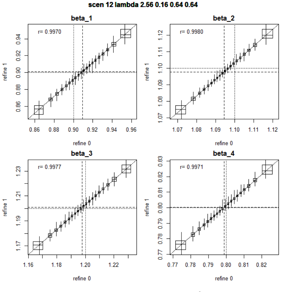
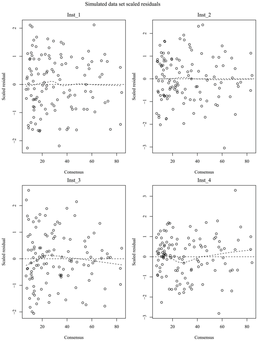
- Figures 1–6 are described as comparative box-and-whisker plots with lowess smooths, but axis labels and the precise meaning of the vertical/horizontal reference lines are only in the text; adding concise figure captions would improve readability.
- The Conclusion notes that all β_i must be positive for the latent μ to be well-defined; a one-sentence remark earlier (near the consensus normalization) would alert readers before the algorithm is presented.
- In the outlier reinclusion stage the text writes “NK” without clarifying that it is n−K; a brief definition would avoid ambiguity.
Circularity Check
No significant circularity: standard parametric extension of two-instrument Deming with independent multi-instrument MLE, residual scaling, and outlier procedure; self-citations supply only the base case.
full rationale
The paper develops a multi-instrument extension of precision-profile-weighted Deming regression. Model (1) posits shared shape g with instrument-specific α_i, β_i, λ_i; the -2 log-likelihood (2)/(5) yields alternating MLE for μ_j (Eq. 3) and weighted least-squares for α, β, with a single λ-refinement step motivated by degeneracy of the likelihood when any λ o0. Scaled residuals (7) follow by substituting fitted parameters into the model variance; the two-stage Mahalanobis/Hotelling outlier screen is a direct application of Rosner ESD and standard multivariate diagnostics. Simulations (Figs 1–6) generate data under known truth and recover essentially unbiased α, β (and usable λ after one refinement); examples diagnose induced and real outliers. Self-citations (1,2,9) supply only the two-instrument base case and the CRAN package; the multi-instrument likelihood, refinement heuristic, residual definition, and outlier algorithm are derived and validated independently inside the paper. No fitted constant is renamed a prediction, no uniqueness theorem is imported to forbid alternatives, and no ansatz is smuggled via citation. The shared-shape assumption is a modeling premise, not a circular step. Score 1 reflects only the ordinary (non-load-bearing) self-citation of the two-instrument precursor.
Assumptions & free parameters
free parameters (5)
- Rocke–Lorenzato κ and ρ (or σ,κ)
- Instrument-specific α_i, β_i, λ_i
- Latent concentrations μ_j
- Number of λ refinement steps (=1)
- Outlier search budget K (default ~5% of n)
assumptions (6)
- domain assumption Assay errors are independent normal with variance λ_i g(α_i+β_i μ_j) and common shape g across instruments.
- domain assumption Precision profile is Rocke–Lorenzato: g(μ)=κ²+ρ²μ² (constant plus proportional components).
- domain assumption All slopes β_i are positive so a common latent μ is identifiable and estimable.
- ad hoc to paper Consensus normalization: average intercept 0 and average slope 1 (egalitarian analysis).
- ad hoc to paper Ignoring second-order log(g) terms when updating μ and when forming scaled residuals is adequate.
- domain assumption Jackknife standard errors are valid for the multi-instrument parameter vector.
Cite this review
Pith. "Pith review of Multiple Instrument Methods Comparison by Precision weighted Deming Regression." pith.science (2026). https://pith.science/paper/5XQXJNBB
@misc{pith2026260711776,
  author       = {Pith},
  title        = {Pith review of: Multiple Instrument Methods Comparison by Precision weighted Deming Regression},
  year         = {2026},
  howpublished = {\url{https://pith.science/paper/5XQXJNBB}},
  note         = {Machine review of arXiv:2607.11776}
}
read the original abstract
In methods comparison (MC) studies, specimens are tested using two or more instruments with the objective of establishing the statistical relationship between the different instruments readings. Unlike regular regression, this is an errors in variables problem. Relationships may be fitted parametrically (Deming regression) or non-parametrically (Passing Bablok or PB regression.) In clinical chemistry settings, the measurement variability is rarely constant, but generally increases with increasing analyte values. Precision weighted Deming regression models this variability and incorporates it into the fitting. The simplest setting of comparing two instruments is discussed in (1) and implemented in an R package (2). PB makes minimal distributional assumptions. Its classical two-instrument implementation has recently been extended to multiple instruments (3). This work extends the two-instrument Deming model of (1) to multiple instruments, developing algorithms for fitting, for formal inference, for residual analysis, and for outlier detection and diagnosis.
Figures


Figures from the paper (7 more)




Reference graph
Works this paper leans on
-
[1]
1 Hawkins DM and Kraker JJ. Precision profile weighted Deming regression for methods comparison, J Appl Lab Med (2026) doi.org/10.1093/jal/jfaf183. 2 Hawkins DM and Kraker JJ. ppwdeming htpps://CRAN.R-project.org/package=ppwdeming 3 Dufey F. Robust regression techniques for multiple method comparison and transformation. Biom J 2024 1-13. 4 Weisberg S. App...
-
[2]
Percentage points for a generalized ESD many-outlier procedure
Chapman and Hall 8 Rosner B. Percentage points for a generalized ESD many-outlier procedure. Technometrics 25 1983 165-172 Multi-instrument precision profile weighted Deming analysis 16 Figure 1 Four instruments’ estimated λ. Multi-instrument precision profile weighted Deming analysis 17 Figure 2 Four instruments’ estimated α. Multi-instrument precision p...
1983
Reviewed July 14, 2026 · model on record in the stance chip above.
Discussion (0). Sign in to comment.