REVIEW 5 major objections 7 minor 51 references
Post-FWI Injection of Learned Priors Using a Flow Matching Model
T0 review · 5 major / 7 minor · reviewed 2026-07-30 · grok-4.5
Pith's one-line read A flow-matching model can refine finished FWI velocity models by injecting learned geological priors and well logs without re-running the inversion.
desk verdict Clean post-FWI flow-matching editor that honestly injects priors; the high-frequency “resolution” is prior content by design, and they never check data fit. read the letter →
The pith
A machine-rendered reading of the paper's core claim, the machinery that carries it, and where it could break.
The reading
What carries the argument
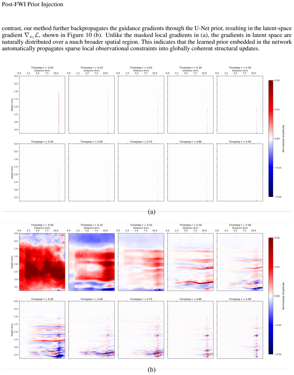
Guided flow matching with latent-variable optimization: at each step the network predicts a clean model from the current latent state; a Gaussian-smoothed comparison to the FWI result and a masked comparison to well logs produce a loss whose gradient updates the latent, so the learned prior carries sparse constraints into a globally coherent sample.
What would settle it
On a field area with an independent high-quality well or borehole image not used in guidance, check whether the refined model reduces depth misties and improves structural match at that well relative to the input FWI without introducing layer or fault patterns that contradict the unused control or the seismic image.
Extended reading notes
Core claim
A post-FWI refinement based on an unconditional flow-matching generative model can inject learned geological priors—and optional well-log constraints—into a provided FWI velocity model by guiding the deterministic generation trajectory in latent space, without additional FWI iterations or explicit seismic data fitting during generation, and thereby improve resolution, suppress artifacts, and raise geological quality, including correcting depth misties toward wells.
Load-bearing premise
That smoothing the generated model is a fair stand-in for what FWI actually recovered, and that the hand-built training ensembles really match the geology of the target field so guidance restores true structure rather than prior-shaped fiction.
Editorial extensions
If this is right
- Finished FWI products can be upgraded with geological priors and wells without access to the original seismic data or another inversion run.
- Choice of training ensemble (thin faulted layers versus thicker continuous layers) directly controls which structures the refinement invents or strengthens.
- Masked well guidance plus the generative prior can propagate sparse log information into laterally continuous high-frequency structure without a separate extrapolation step.
- Frequency-split joint constraints can reconcile smooth FWI backgrounds with high-wavenumber well detail when full-band joint fitting is unstable.
- The same post-process framing can later carry other high-resolution constraints (for example near-surface seismic) into a vendor FWI model.
Reading between the lines
- If the method is reliable, operators could maintain a library of regional geological prior models and apply them as a standard QC or handoff step on any incoming FWI cube.
- Visible sensitivity to which prior class is chosen implies the workflow needs a transparent prior-selection protocol, not a single universal generative model.
- Because generation never re-enforces the wave equation, a natural next test is whether the refined model still explains the original seismic data within noise, or systematically drifts off the data manifold.
- Correcting depth misties post hoc may reduce the need to re-run anisotropic FWI solely to honor wells, but only if the mistie cause is velocity structure the prior can represent.
Editorial analysis
A structured set of objections, weighed in public.
Referee Report
Summary. The manuscript proposes a flow-matching post-processing method for an already-computed FWI velocity model. An unconditional or class-conditional FM model is trained on synthetic geological ensembles; during deterministic generation, latent states are optimized so that a Gaussian-smoothed prediction matches the FWI model and, optionally, a masked or high-pass-filtered prediction matches well logs. The approach is applied to an Otway synthetic example and to CGG and Viking field data. The authors report artifact suppression, sharper layers and faults, propagation of well information, and possible correction of depth misties without additional FWI iterations or direct seismic-data fitting during generation.
Significance. If validated, the method could be practically useful: it offers a clear way to modify vendor-supplied or otherwise finalized FWI models using geological ensembles and sparse wells without rerunning the wave-equation inversion. Strengths include a coherent deterministic FM formulation, an explicit latent-optimization algorithm, the low-pass/masking construction, and demonstrations at both synthetic and field scale. The method is deliberately not parameter-free, however, and its present evidence does not yet establish that injected detail is geologically correct or seismic-data consistent.
major comments (5)
- [§3.3, Eqs. (8)–(14)] §3.3.1, Eqs. (8)–(10), and §3.3.2, Eq. (14): with the stated convention x0~p0 (Gaussian) and x1~pdata, differentiation of Eq. (8) gives v*=x1-x0, not x0-x1. Likewise, differentiation of Eq. (11) gives I+(1-t)∂vθ/∂xt, whereas Eq. (14) has a minus sign. Algorithm 1 integrates xt+vθΔt toward increasing t and therefore appears consistent with v*=x1-x0. Please correct the signs or explicitly reverse and consistently restate the x0/x1 convention; these signs determine both the trajectory direction and the guidance gradient.
- [§3.4.1, Eq. (15); §4.3–4.4] The FWI guidance loss constrains only Gσ*x̂1 against xFWI. Consequently, spectral content outside the effective Gaussian passband is supplied by the learned prior and the optimization hyperparameters, not by seismic information. This makes the broad claim of 'resolution enhancement' ambiguous: Figs. 6 and 11 already show that changing the prior changes faults and continuity. A mismatched-prior/null-prior test on an independent synthetic case, together with spectral error analysis showing which wavenumbers track truth and which merely follow the prior, is needed to distinguish recovered structure from prior-consistent hallucination.
- [§4.1–4.2, Figs. 4–5] The Otway prior ensemble is 'extracted from the Otway model' that also provides the ground truth in Fig. 4. The manuscript does not state whether the target model, nearby patches, or statistically equivalent fault realizations were excluded from training. The claimed fault recovery could therefore partly reflect training-set recall. Please document the train/validation/test construction, use a genuinely held-out geological realization (or independently generated ensemble), describe the FWI acquisition and frequency setup, and report quantitative errors and variability over random initializations.
- [§3.4.2–3.4.3; §4.3–4.4] Equations (19)–(21) explicitly minimize disagreement at the guided well locations, so the improved agreement shown at those same locations in Figs. 8(c,e) and 12(c,e) is a fitting diagnostic rather than independent validation. In particular, the abstract's claim of correcting depth misties requires evidence that the induced depth shift is physically correct: for example, a synthetic test with a known mistie, leave-one-well-out validation, or verification against an independent well or marker. The roles of the F3 cutoff, anisotropy, and depth conversion should also be separated from the claimed correction.
- [§4, data consistency] No experiment checks that the refined velocity model still explains the recorded seismic data. Because the refinement can also alter components within the Gaussian passband—and freely alters higher wavenumbers—it may move away from the FWI model's data-consistent solution. At minimum, forward-model the refined result using the same synthetic physics and compare shot-record residuals with those of the FWI baseline; a field-data check should be added if the data are available. If such a check is outside scope, the contribution should be framed as prior-conditioned model editing, not as an improved FWI solution.
minor comments (7)
- [General] There are several typographical or terminology issues: 'startegies' in §3.4.2, 'otway prior' later in §4.3, repeated 'Equation. 20', and the reference to 'Algorithm 14' in §3.4. Section 4.2 also calls the integration from ts to T the 'reverse process', although t increases.
- [§3.4 and Algorithm 1] Notation alternates among x1, m, xFWI, mwell, and xwell. Please state whether xwell is a one-dimensional log or a spatially embedded image, define its interpolation and normalization, and use ˆx1 consistently in Eqs. (20)–(21).
- [§4.1–4.4] For reproducibility, report the values or selection procedure for σ, λ1, λ2, the F3 cutoff, guidance step size, and random seeds for each experiment. The U-Net size, parameter count, normalization, augmentation, and exact procedure used to generate 5,000 samples from each prior family are also not fully specified.
- [§4.3] The field examples process 608×608 models with a network trained on 320×304 samples. Please clarify whether this relies on the U-Net being fully convolutional, whether padding or boundary artifacts arise, and how stable the result is to initialization and crop position.
- [Figures 4–12] Several claims depend on arrows and visually selected regions. Add colorbars with units, label all profile curves explicitly, and consider difference panels or quantitative profile errors so readers can assess the changes without relying on figure annotations.
- [§4.3, Fig. 9] The discussion of Fig. 9 refers to a 'diffusion prior', although the method is presented as flow matching. Please use consistent terminology, especially because the introduction emphasizes the distinction between FM and diffusion models.
- [References] References [45] and [47] appear to cite the same Plug-and-Play paper in two venues. Please consolidate them and check the publication status and formatting of the arXiv and conference references.
Circularity Check
Mild framing circularity: well-match and prior-shaped geology are partly success-by-construction; the FM post-FWI method itself is not a self-defining derivation.
-
self definitional
[Abstract; §3.4.2 Eqs. 17–19; joint loss Eqs. 20–21]
"In fact, the well prior even managed to alter the model depth to fit the well information, which is a form of correcting for depth misties. ... F2(x̂1)=M⊙x̂1 ... Lwell=∥F2(x̂1)−mwell∥2 ... L=λ1∥F1(x̂)−xFWI∥22+λ2∥M⊙x̂−xwell∥22"
The well term is an explicit least-squares match of the generated model to the well log at masked locations. Optimizing that loss necessarily pulls the model (including depth) toward the well. Presenting post-optimization well agreement / depth shift as empirical ‘correction of depth misties’ treats constraint satisfaction as an independent discovery. The demonstration reduces to the definition of the guidance objective.
-
fitted input called prediction
[§4.1 Datasets and Training; §4.2 Otway synthetic (Fig. 4)]
"Two representative geological prior datasets are prepared: Otway priors (extracted from the Otway model which belongs to Stage 2C of the Otway project by CO2CRC Limited [49], Figure 2 (a)) ... Figure 4 (c) shows the predicted sample using the learned Otway priors under the guidance of the FWI result ... As highlighted by the arrows, the faults have been clearly recovered."
The Otway FM prior is built from samples extracted from the Otway model, and the synthetic test uses that same model family as ground truth. Fault structures the network was trained to reproduce are then reported as ‘recovered’ under Otway-prior guidance. The synthetic success metric is partly contaminated by training-set content rather than a fully held-out geological target.
1 more flagged steps
-
self definitional
[§4.1; field evaluation §4.3–4.4 (Figs. 6, 7, 11)]
"CGG priors (we refer to it CGG because it reflects what we expect the Earth model corresponding to the CGG data would look like, Figure 2 (b)). ... When the CGG priors are injected, the layers become more laterally continuous in a geologically meaningful manner ... the result generated using the CGG prior exhibits more geologically plausible layer continuations"
The CGG training ensemble is defined as the authors’ expected geology for that field. Field success is then largely scored by visual geological plausibility and continuity that match those same expectations (and switches when the Otway prior is used instead). ‘Geological quality’ is therefore measured against the prior that was injected, not against an independent external label or held-out seismic misfit—so the quality claim is partly self-referential.
full rationale
This is a methods paper, not a first-principles derivation of a physical law. Flow matching is trained on external ensembles, then the latent trajectory is guided toward an externally supplied FWI cube and optional wells. That pipeline is not equivalent to its inputs by definition: the generative prior can (and does) add structure not present in the FWI result, and different priors produce visibly different outputs (Otway vs CGG). No load-bearing uniqueness theorem or self-citation chain forces the central claim. Two milder circularities remain in how results are sold. (1) Well ‘depth-mistie correction’ is largely the well-guidance loss doing what it is written to do (mask match at well locations), so reporting post-guidance well agreement as an independent correction is partly tautological. (2) Field ‘geological quality’ is judged against the same hand-built expectations used to construct the CGG/Otway training priors, and the Otway synthetic prior is extracted from the same model family used as ground truth—so synthetic fault ‘recovery’ and field prior-likeness are not fully external benchmarks. These weaken the validation narrative but do not collapse the method into a definitional identity. Score 3 reflects partial success-by-construction in the well and prior-evaluation stories, not circularity of the algorithm.
Assumptions & free parameters
free parameters (5)
- Gaussian smoothing scale σ in F1 =
not numerically reported; adjusted per FWI resolution
- Guidance weights λ1, λ2
- Generation schedule T, start step ts, inner steps N =
T=100; ts=50 (Otway) / 30 (field); N=1
- Prior class / training ensemble choice (Otway vs CGG-style) =
class-conditional FM on 5000 samples per prior type
- High-pass filter F3 for frequency-decomposed well loss
assumptions (5)
- domain assumption Linear-interpolation flow matching with velocity field vθ learns a usable prior over high-resolution velocity models from finite synthetic ensembles.
- ad hoc to paper A Gaussian convolution adequately approximates the forward map from a high-resolution plausible model to an FWI result for guidance purposes.
- domain assumption Sparse well constraints applied only through a mask, backpropagated through the U-Net, suffice for globally consistent geological updates without explicit spatial extrapolation.
- domain assumption Decoupling data misfit from regularization into a pure post-process still yields models that remain acceptable for the original seismic experiment.
- standard math Standard calculus / ODE integration and ℓ2 guidance losses are valid.
invented entities (1)
-
Smoothed-FWI + masked-well latent guidance recipe for unconditional FM post-FWI refinement
Cite this review
Pith. "Pith review of Post-FWI Injection of Learned Priors Using a Flow Matching Model." pith.science (2026). https://pith.science/paper/GZI2K2WV
@misc{pith2026260723719,
  author       = {Pith},
  title        = {Pith review of: Post-FWI Injection of Learned Priors Using a Flow Matching Model},
  year         = {2026},
  howpublished = {\url{https://pith.science/paper/GZI2K2WV}},
  note         = {Machine review of arXiv:2607.23719}
}
read the original abstract
Full Waveform Inversion (FWI) is a powerful tool for subsurface velocity reconstruction but remains highly ill-posed, sensitive to acquisition limitations, often requiring some form of regularization to reduce artifacts and enhance resolution. While recent developments have shown that generative models can inject learned priors directly into the FWI optimization process, such approaches typically require additional, computationally expensive inversion iterations. In this study, we propose a post-FWI refinement strategy based on a Flow Matching (FM) generative model, which leverages learned geological priors without re-running FWI. The method guides the deterministic generative process using the FWI result, as well as well logs, if available. Synthetic and field data experiments demonstrate that we can inject well information and our geological expectations (prior) into the provided FWI result, and thus, we can effectively enhance its resolution and geological quality. In fact, the well prior even managed to alter the model depth to fit the well information, which is a form of correcting for depth misties.
Figures


Figures from the paper (10 more)




Reference graph
Works this paper leans on
-
[1]
An overview of full-waveform inversion in exploration geophysics.Geophysics, 74(6):WCC1–WCC26, 2009
Jean Virieux and Stéphane Operto. An overview of full-waveform inversion in exploration geophysics.Geophysics, 74(6):WCC1–WCC26, 2009
2009
-
[2]
Well-to-seismic mistie: A valuable indicator of seismic anisotropy for subsalt velocity model update
Huyen Bui, Peck Hwa David Ng, David Becker, Zhengyun Zhou, and Martiris Smith. Well-to-seismic mistie: A valuable indicator of seismic anisotropy for subsalt velocity model update. a case study in a deviated subsalt well in the deepwater gulf of mexico. InSEG International Exposition and Annual Meeting, pages SEG–2010. SEG, 2010
2010
-
[3]
Well-to-seismic tie
Gerardo Clemente Martínez, Grant Hanson, Hammad Hassan Tariq, Jaap Van der Toorn, Jose Adauto de Souza, Matthijs van der Molen, Oleksandr Okprekyi, Rajeshwaran Dandapani, and Zaheer Ali Shah. Well-to-seismic tie. InApplied techniques to integrated oil and gas reservoir characterization, pages 249–271. Elsevier, 2021
2021
-
[4]
Edge-preserving and scale-dependent properties of total variation regularization
David Strong and Tony Chan. Edge-preserving and scale-dependent properties of total variation regularization. Inverse problems, 19(6):S165, 2003
2003
-
[5]
Constrained full-waveform inversion by model reparameteri- zation.Geophysics, 77(2):R117–R127, 2012
Antoine Guitton, Gboyega Ayeni, and Esteban Díaz. Constrained full-waveform inversion by model reparameteri- zation.Geophysics, 77(2):R117–R127, 2012
2012
-
[6]
Tikhonov regularization and total least squares
Gene H Golub, Per Christian Hansen, and Dianne P O’Leary. Tikhonov regularization and total least squares. SIAM journal on matrix analysis and applications, 21(1):185–194, 1999. 15 Post-FWI Prior Injection
1999
-
[7]
Regularized seismic full waveform inversion with prior model information.Geophysics, 78(2):R25–R36, 2013
Amir Asnaashari, Romain Brossier, Stéphane Garambois, François Audebert, Pierre Thore, and Jean Virieux. Regularized seismic full waveform inversion with prior model information.Geophysics, 78(2):R25–R36, 2013
2013
-
[8]
Synthetic inversions for density using seismic and gravity data.Geophysical Journal International, 209(2):1204–1220, 2017
Nienke Blom, Christian Boehm, and Andreas Fichtner. Synthetic inversions for density using seismic and gravity data.Geophysical Journal International, 209(2):1204–1220, 2017
2017
Show all 51 references
-
[9]
Regularized elastic full-waveform inversion using deep learning
Zhen-Dong Zhang and Tariq Alkhalifah. Regularized elastic full-waveform inversion using deep learning. GEOPHYSICS, 84:R741–R751, 2019
2019
-
[10]
Deep-learning assisted regularized elastic full waveform inversion using the velocity distribution information from wells.Geophysical Journal International, 226(2):1322– 1335, 2021
Yuanyuan Li, Tariq Alkhalifah, and Zhendong Zhang. Deep-learning assisted regularized elastic full waveform inversion using the velocity distribution information from wells.Geophysical Journal International, 226(2):1322– 1335, 2021
2021
-
[11]
Full-waveform inversion using a learned regularization.IEEE Transactions on Geoscience and Remote Sensing, 61:1–15, 2023
Pengpeng Sun, Fangshu Yang, Hongxian Liang, and Jianwei Ma. Full-waveform inversion using a learned regularization.IEEE Transactions on Geoscience and Remote Sensing, 61:1–15, 2023
2023
-
[12]
Alkhalifah
Fu Wang, Xinquan Huang, and Tariq A. Alkhalifah. A prior regularized full waveform inversion using generative diffusion models.IEEE Transactions on Geoscience and Remote Sensing, 61:1–11, 2023
2023
-
[13]
Full-waveform inversion with denoising priors based on graph space sinkhorn distance.IEEE Transactions on Geoscience and Remote Sensing, 63:1–13, 2025
Zhoujie Tan, Gang Yao, Feng Zhang, and Di Wu. Full-waveform inversion with denoising priors based on graph space sinkhorn distance.IEEE Transactions on Geoscience and Remote Sensing, 63:1–13, 2025
2025
-
[14]
Deep learning prior models from seismic images for full-waveform inversion
Winston Lewis and Denes Vigh. Deep learning prior models from seismic images for full-waveform inversion. In SEG international exposition and annual meeting, pages SEG–2017. SEG, 2017
2017
-
[15]
Conditional image prior for uncertainty quantification in full-waveform inversion
Lingyun Yang, Omar M Saad, Tariq Alkhalifah, and Guochen Wu. Conditional image prior for uncertainty quantification in full-waveform inversion. InSEG International Exposition and Annual Meeting, pages SEG–2024. SEG, 2024
2024
-
[16]
Reparameterized full-waveform inversion using deep neural networks.Geophysics, 86(1):V1–V13, 2021
Qinglong He and Yanfei Wang. Reparameterized full-waveform inversion using deep neural networks.Geophysics, 86(1):V1–V13, 2021
2021
-
[17]
Elastic full-waveform inversion using a physics-guided deep convolutional encoder–decoder.IEEE Transactions on Geoscience and Remote Sensing, 61:1–18, 2023
Arnab Dhara and Mrinal K Sen. Elastic full-waveform inversion using a physics-guided deep convolutional encoder–decoder.IEEE Transactions on Geoscience and Remote Sensing, 61:1–18, 2023
2023
-
[18]
Multiscale neural decoding and weighting for reparameterized seismic full-waveform inversion.Geophysics, 91(2):R65–R80, 2026
Yufeng Wang, Ning Gan, Shaohua Zhang, Weiguang He, Xueming Shi, and Xiangyun Hu. Multiscale neural decoding and weighting for reparameterized seismic full-waveform inversion.Geophysics, 91(2):R65–R80, 2026
2026
-
[19]
Bayesian full-waveform inversion with realistic priors.Geophysics, 86(5):A45– A49, 2021
Xin Zhang and Andrew Curtis. Bayesian full-waveform inversion with realistic priors.Geophysics, 86(5):A45– A49, 2021
2021
-
[20]
Bayesian variational time-lapse full waveform inversion.Geophysical Journal International, 237(3):1624–1638, 2024
Xin Zhang and Andrew Curtis. Bayesian variational time-lapse full waveform inversion.Geophysical Journal International, 237(3):1624–1638, 2024
2024
-
[21]
Plug and play post-stack seismic inversion with cnn-based denoisers
Juan Romero, Miguel Corrales, Nicolaas Luiken, and Matteo Ravasi. Plug and play post-stack seismic inversion with cnn-based denoisers. InSecond EAGE subsurface intelligence workshop, volume 2022, pages 1–5. European Association of Geoscientists & Engineers, 2022
2022
-
[22]
Plug-and-play regularized multi-dimensional deconvolution for accurate wavefield retrieval and imaging
Ning Wang and Tariq Alkhalifah. Plug-and-play regularized multi-dimensional deconvolution for accurate wavefield retrieval and imaging. 2026
2026
-
[23]
Self-supervised pre-training vision transformer with masked autoencoders for building subsurface model.IEEE Transactions on Geoscience and Remote Sensing, 2023
Yuanyuan Li, Tariq Alkhalifah, Jianping Huang, and Zhenchun Li. Self-supervised pre-training vision transformer with masked autoencoders for building subsurface model.IEEE Transactions on Geoscience and Remote Sensing, 2023
2023
-
[24]
Velocity model building and editing with guided denoising diffusion implicit models.arXiv preprint arXiv:2603.01231, 2026
Francesco Brandolin and Tariq Alkhalifah. Velocity model building and editing with guided denoising diffusion implicit models.arXiv preprint arXiv:2603.01231, 2026
2026 arXiv
-
[25]
Flow matching for generative modeling.arXiv preprint arXiv:2210.02747, 2022
Yaron Lipman, Ricky TQ Chen, Heli Ben-Hamu, Maximilian Nickel, and Matt Le. Flow matching for generative modeling.arXiv preprint arXiv:2210.02747, 2022
2022 arXiv
-
[26]
Flow straight and fast: Learning to generate and transfer data with rectified flow.arXiv preprint arXiv:2209.03003, 2022
Xingchao Liu, Chengyue Gong, and Qiang Liu. Flow straight and fast: Learning to generate and transfer data with rectified flow.arXiv preprint arXiv:2209.03003, 2022
2022 arXiv
-
[27]
Scaling rectified flow transformers for high-resolution image synthesis
Patrick Esser, Sumith Kulal, Andreas Blattmann, Rahim Entezari, Jonas Müller, Harry Saini, Yam Levi, Dominik Lorenz, Axel Sauer, Frederic Boesel, et al. Scaling rectified flow transformers for high-resolution image synthesis. InForty-first international conference on machine l...
2024
-
[28]
Diffusion model for das-vsp data denoising.Sensors, 23(20):8619, 2023
Donglin Zhu, Lei Fu, Vladimir Kazei, and Weichang Li. Diffusion model for das-vsp data denoising.Sensors, 23(20):8619, 2023
2023
-
[29]
Conditional denoising diffusion probabilistic model for seismic diffraction separation and imaging.IEEE Transactions on Geoscience and Remote Sensing, 62:1–13, 2024
Hao Zhang, Yuanyuan Li, and Jianping Huang. Conditional denoising diffusion probabilistic model for seismic diffraction separation and imaging.IEEE Transactions on Geoscience and Remote Sensing, 62:1–13, 2024. 16 Post-FWI Prior Injection
2024
-
[30]
Conditional denoising diffusion probabilistic model for ground-roll attenuation.arXiv preprint arXiv:2403.18224, 2024
Yuanyuan Li, Hao Zhang, Jianping Huang, and Zhenchun Li. Conditional denoising diffusion probabilistic model for ground-roll attenuation.arXiv preprint arXiv:2403.18224, 2024
2024 arXiv
-
[31]
Posterior sampling for random noise attenuation via score-based generative models.Geophysics, 90(2):1–54, 2024
Chuangji Meng, Jinghuai Gao, Baohai Wu, Hongling Chen, and Yajun Tian. Posterior sampling for random noise attenuation via score-based generative models.Geophysics, 90(2):1–54, 2024
2024
-
[32]
Geological and well prior assisted full waveform inversion using conditional diffusion models
Fu Wang and T Alkhalifah. Geological and well prior assisted full waveform inversion using conditional diffusion models. In85th EAGE Annual Conference & Exhibition (including the Workshop Programme), volume 2024, pages 1–5. European Association of Geoscientists & Engineers, 2024
2024
-
[33]
Diffusionvel: Multi-information integrated velocity inversion using generative diffusion models.arXiv preprint arXiv:2410.21776, 2024
Hao Zhang, Yuanyuan Li, and Jianping Huang. Diffusionvel: Multi-information integrated velocity inversion using generative diffusion models.arXiv preprint arXiv:2410.21776, 2024
2024 arXiv
-
[34]
Multi-diffusioninv: Prior-based multi-constraint full wave inversion by generative diffusion models
H Zhang, Y Li, J Huang, and G Li. Multi-diffusioninv: Prior-based multi-constraint full wave inversion by generative diffusion models. In86th EAGE Annual Conference & Exhibition, volume 2025, pages 1–5. European Association of Geoscientists & Engineers, 2025
2025
-
[35]
Well-and structure-constrained initial velocity building for full-waveform inversion via a generative diffusion model.IEEE Transactions on Geoscience and Remote Sensing, 2025
Qingchen Zhang, Shijun Cheng, Wei Chen, and Weijian Mao. Well-and structure-constrained initial velocity building for full-waveform inversion via a generative diffusion model.IEEE Transactions on Geoscience and Remote Sensing, 2025
2025
-
[36]
Sit: Exploring flow and diffusion-based generative models with scalable interpolant transformers
Nanye Ma, Mark Goldstein, Michael S Albergo, Nicholas M Boffi, Eric Vanden-Eijnden, and Saining Xie. Sit: Exploring flow and diffusion-based generative models with scalable interpolant transformers. InEuropean Conference on Computer Vision, pages 23–40. Springer, 2024
2024
-
[37]
Diff2flow: Training flow matching models via diffusion model alignment
Johannes Schusterbauer, Ming Gui, Frank Fundel, and Björn Ommer. Diff2flow: Training flow matching models via diffusion model alignment. InProceedings of the Computer Vision and Pattern Recognition Conference, pages 28347–28357, 2025
2025
-
[38]
Controllable seismic velocity synthesis using generative diffusion models.Journal of Geophysical Research: Machine Learning and Computation, 1(3):e2024JH000153, 2024
Fu Wang, Xinquan Huang, and Tariq Alkhalifah. Controllable seismic velocity synthesis using generative diffusion models.Journal of Geophysical Research: Machine Learning and Computation, 1(3):e2024JH000153, 2024
2024
-
[39]
Diffusion model-based posterior sampling in full waveform inversion
Mohammad H Taufik and Tariq Alkhalifah. Diffusion model-based posterior sampling in full waveform inversion. arXiv preprint arXiv:2512.12797, 2025
2025
-
[40]
Proximal algorithms.Foundations and Trends in Optimization, 1(3):127–239, 2014
Neal Parikh and Stephen Boyd. Proximal algorithms.Foundations and Trends in Optimization, 1(3):127–239, 2014
2014
-
[41]
A fast iterative shrinkage-thresholding algorithm for linear inverse problems
Amir Beck and Marc Teboulle. A fast iterative shrinkage-thresholding algorithm for linear inverse problems. SIAM Journal on Imaging Sciences, 2(1):183–202, 2009
2009
-
[42]
Regularized full-waveform inversion with automated salt flooding.Geophysics, 84(4):R569–R582, 2019
Mahesh Kalita, Vladimir Kazei, Yunseok Choi, and Tariq Alkhalifah. Regularized full-waveform inversion with automated salt flooding.Geophysics, 84(4):R569–R582, 2019
2019
-
[43]
An accelerated proximal gradient algorithm for source-independent waveform inversion.Journal of Applied Geophysics, 177:104030, 2020
Hongsun Fu, Mingyue Ma, and Bo Han. An accelerated proximal gradient algorithm for source-independent waveform inversion.Journal of Applied Geophysics, 177:104030, 2020
2020
-
[44]
Distributed optimization and statistical learning via the alternating direction method of multipliers.Foundations and Trends in Machine Learning, 3(1):1–122, 2011
Stephen Boyd, Neal Parikh, Eric Chu, Borja Peleato, and Jonathan Eckstein. Distributed optimization and statistical learning via the alternating direction method of multipliers.Foundations and Trends in Machine Learning, 3(1):1–122, 2011
2011
-
[45]
Venkatakrishnan, Charles A
Singanallur V . Venkatakrishnan, Charles A. Bouman, and Brendt Wohlberg. Plug-and-play priors for model based reconstruction. In2013 IEEE Global Conference on Signal and Information Processing, pages 945–948, 2013
2013
-
[46]
Taufik, Fu Wang, and Tariq Alkhalifah
Mohammad H. Taufik, Fu Wang, and Tariq Alkhalifah. Learned regularizations for multi-parameter elastic full waveform inversion using diffusion models.Journal of Geophysical Research: Machine Learning and Computation, 1(1):e2024JH000125, 2024
2024
-
[47]
Venkatakrishnan, Charles A
Singanallur V . Venkatakrishnan, Charles A. Bouman, and Brendt Wohlberg. Plug-and-play priors for model based reconstruction. InIEEE Global Conference on Signal and Information Processing, 2013
2013
-
[48]
The little engine that could: Regularization by denoising (red).SIAM Journal on Imaging Sciences, 10(4):1804–1844, 2017
Yaniv Romano, Michael Elad, and Peyman Milanfar. The little engine that could: Regularization by denoising (red).SIAM Journal on Imaging Sciences, 10(4):1804–1844, 2017
2017
-
[49]
Seismic monitoring of co2 geosequestration: Co2crc otway case study using full 4d fdtd approach
Stas Glubokovskikh, Roman Pevzner, Tess Dance, Eva Caspari, Dmitry Popik, Valeriya Shulakova, and Boris Gurevich. Seismic monitoring of co2 geosequestration: Co2crc otway case study using full 4d fdtd approach. International Journal of Greenhouse Gas Control, 49:201–216, 2016
2016
-
[50]
High-resolution image synthesis with latent diffusion models
Robin Rombach, Andreas Blattmann, Dominik Lorenz, Patrick Esser, and Björn Ommer. High-resolution image synthesis with latent diffusion models. InProceedings of the IEEE/CVF conference on computer vision and pattern recognition, pages 10684–10695, 2022. 17 Post-FWI Prior Injection
2022
-
[51]
Bingbing Sun and Tariq Alkhalifah. An anisotropic waveform inversion using an optimal transport matching filter objective: An application to an offshore field dataset.IEEE Transactions on Geoscience and Remote Sensing, 61:1–22, 2023. 18
2023
Reviewed July 30, 2026 · model on record in the stance chip above.
Discussion (0). Continue with ORCID to comment.