REVIEW 3 major objections 8 minor 24 references
Density-Robust Spherical Coordinates from Persistent Cohomology
T0 review · 3 major / 8 minor · reviewed 2026-07-31 · grok-4.5
Pith's one-line read The first density-robust spherical coordinates from persistent cohomology are built by computing classical sphere maps on rejection-sampled uniform subsamples and aligning them with a spherical Procrustes problem.
desk verdict Solid first density-robust S² pipeline via subsample-and-Procrustes; math is clean, robustness still empirical and only synthetic. read the letter →
The pith
A machine-rendered reading of the paper's core claim, the machinery that carries it, and where it could break.
The reading
What carries the argument
The spherical Procrustes problem (jointly rotating several S²-valued maps and choosing a consensus map to minimize summed squared geodesic discrepancy), together with Theorem 3.4, which bounds the distance between the Euclidean O(3) Procrustes solution (projected back to the sphere) and the true spherical optimum by (1+π) times the square root of the minimal spherical loss.
What would settle it
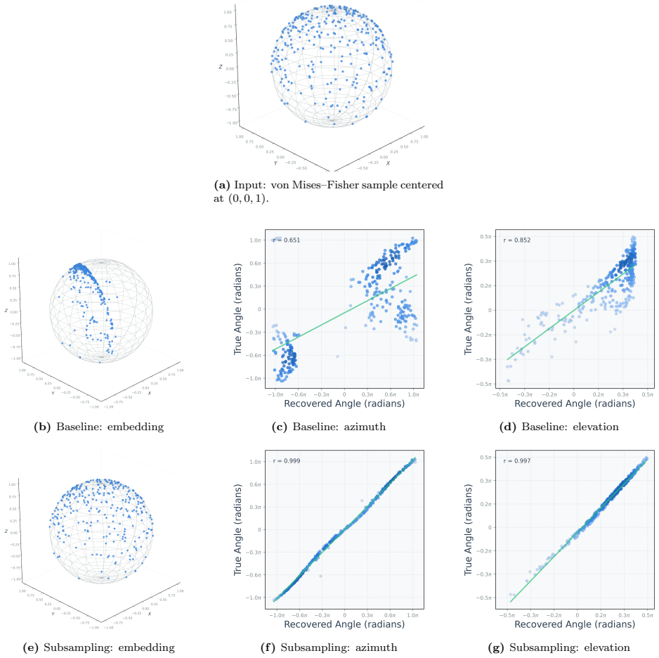
Take a sphere sampled from a strongly biased density (for example von Mises–Fisher with large concentration), run the full subsample-align-average pipeline with the paper’s density estimator, and check whether recovered azimuth and elevation still correlate tightly with ground truth; a clear systematic warp that survives many subsamples and alignments would refute the claim.
Extended reading notes
Core claim
Density-robust spherical topological coordinates exist and can be constructed by extending the subsampling-and-alignment paradigm from the circle to the sphere: compute classical spherical coordinates on approximately uniform rejection samples, extend them by kernel-weighted nearest neighbors, and combine them by solving a spherical Procrustes problem whose Euclidean relaxation approximates the intrinsic optimum within a factor controlled by the optimal spherical loss.
Load-bearing premise
That local-count rejection sampling really produces subsamples on which the classical sphere-map optimizer is already unbiased, so that extending and averaging those maps yields a faithful global coordinate.
Editorial extensions
If this is right
- Sphere-valued latent structure can be recovered from data whose observation density is badly non-uniform without rewriting the underlying energy.
- Degree-two persistent cohomology becomes practical on datasets of several thousand to ten thousand points because cohomology is run only on fixed-size subsamples.
- The same alignment idea supplies a template for density-robust coordinates targeting other spaces once a Procrustes-type alignment on that space is available.
- Under uniform sampling the method matches classical spherical coordinates, so it can replace the baseline without quality loss when density is unknown.
Reading between the lines
- Because S² is CP¹, the same subsample-and-align pattern is a natural first step toward density-robust projective coordinates from higher cohomology.
- If the density estimator fails on outliers, a more stable density model (or explicit outlier rejection) would be the highest-leverage practical upgrade before chasing tighter Procrustes bounds.
- The (1+π)√L* guarantee is useful mainly when the spherical loss is already small; experiments that report L* alongside angle error would make the theory–practice link sharper.
Signed reviews
Editorial analysis
A structured set of objections, weighed in public.
Referee Report
Summary. The manuscript constructs the first density-robust spherical (degree-two) coordinates from persistent cohomology. The strategy ports the subsampling-and-alignment framework of Blumberg et al. [4] from S^1 to S^2: rejection sampling against a local-count density estimator produces approximately uniform subsamples, the Schonsheck–Schonsheck spherical coordinate is computed on each, kernel-extended to the full dataset, and the maps are aligned and averaged. The new mathematical content is a spherical Procrustes formulation (Def. 3.2) and an approximation theorem (Thm. 3.4, via the great-circle reduction Lem. 3.3) showing the Euclidean O(3) Procrustes solution, projected back to S^2, lies within (1+π)√L* of the geodesic optimum. Experiments show: two implementation accelerations give >100× speedup of the baseline; subsampling removes the O(n^4) memory ceiling and runs at near-constant cost to 10,000 points; under uniform sampling the method matches the baseline, and under von Mises–Fisher and other biased sampling it recovers azimuth/elevation where the baseline fails. Code and reproduction scripts are public.
Significance. If the empirical robustness holds up, this closes a genuine gap: density-robust topological coordinates existed only in degree one, and the authors correctly explain why the weighted-harmonic-cocycle mechanism of Paik–Park does not transfer to the sphere-valued variational problem. The paper has real strengths that should be credited: Lemma 3.3 and Theorem 3.4 are clean, correctly proved, and the great-circle reduction is a neat observation; the spherical Procrustes formulation is a natural contribution in its own right; the scalability results (removal of the quartic memory bottleneck, near-constant runtime to 10^4 points) are practically important for the degree-two pipeline; and the authors ship a public implementation with fixed seeds, five-trial runtime means, and scripts reproducing all figures. The limitations section (§5) is unusually candid about what is not proved. The main caveats concern the evidentiary basis of the headline robustness claim, which is currently qualitative, and the regime in which Theorem 3.4 is informative.
major comments (3)
- [§4.3, Figs. 5–7] §4.3: the central empirical claim — accurate azimuth/elevation recovery under severe sampling bias — is supported only by scatter-plot figures (Figs. 5–7) at a single configuration each. No numerical error metric is reported: the protocol says coordinates are evaluated 'by correlating' angles against ground truth, but no correlation values or angular errors appear anywhere. The baseline's failure in Fig. 6 is likewise asserted visually. Since robustness is the paper's headline result, I ask for a quantitative table (e.g., circular correlation and/or mean absolute angular error for azimuth and elevation) for baseline vs. subsampling across the uniform, vMF κ=1.3, and the three severe-bias regimes, with variability over seeds and over the subsampling parameters (M, subsample size). This is feasible with the released code and would substantially strengthen the claim.
- [§3.1, §4.3] §4.3 ('Robustness to non-uniform sampling') and §3.1: the mechanism argument — that on each rejection-sampled subsample the Möbius-centering constraint is 'essentially satisfied already,' so per-subsample coordinates are unbiased — is heuristic, and nothing quantifies the residual non-uniformity of the subsamples or relates it to per-subsample coordinate bias. Theorem 3.1 is asymptotic (ε_n→0, ε_n n^{1/(2m)}→∞) and gives no guidance at the n=250–1500 used; the text never states how ε and the acceptance scale C are chosen in the experiments. At minimum, report a subsample-uniformity diagnostic (e.g., the distribution of local counts or estimated density after acceptance) alongside the coordinate errors, and state the estimator parameters used per experiment. If the causal story ('rejection sampling restores uniformity, hence coordinates are unbiased') is to be kept, it needs this quantita
- [§3.2, Thm. 3.4 and proof] Theorem 3.4 is correct as proved, but its informativeness regime should be stated. On S^2 the trivial diameter bound d ≤ π always holds, so (1+π)√L* is non-vacuous only when L* < (π/(1+π))^2 ≈ 0.58 rad², i.e., mean squared geodesic misalignment below about 0.76 rad RMS. Nothing in the paper bounds L* a priori, and in the severe-bias regimes of Fig. 7 — where per-subsample coordinates are computed on 75–120 points and kernel-extended — L* could plausibly approach this threshold. This does not undermine the theorem's purpose (justifying the Euclidean initialization for the subsequent SO(3) refinement), but the paper should (i) state the non-vacuity condition explicitly, and (ii) report the empirical L* (or the bound value) in the experiments so readers can see the guarantee is operative where invoked. Relatedly, the metric d_{(S^2)^n} and d_{(R^3)^n} on configuration space are never define
minor comments (8)
- [§3.2] Proof of Thm. 3.4: 'by the triangle inequality and Theorem 3.3' should read Lemma 3.3 (there is no Theorem 3.3).
- [§3.2 / §4.1] Def. 3.2 restricts rotations to SO(3), but the Euclidean relaxation is solved over O(3) (ten Berge), which includes improper rotations. The theorem legitimately compares against the O(3) optimum, but the initialization passed to the SO(3) refinement may be a reflection; a sentence on how this is handled in practice would help.
- [§3.1] Notation inconsistency in §3.1: the kernel-average formula defines Φ_i, but the following sentence refers to 'unit vectors ϕ_i(y)'. Also 'an Euclidean relaxation' (p. 14) and mixed ϵ/ε throughout.
- [§3.2] Lem. 3.3 cites 'Lemma 4.3 of [4]', an arXiv preprint whose numbering may shift between versions; give the version number or restate the one-dimensional estimate (it is a line or two) for self-containedness.
- [§4.2] Figure 4 appears in the float sequence but is never discussed in the text of §4.2 beyond the caption; either integrate it (which configurations dominate runtime?) or cut it.
- [§4.3] §4.3 opening: 'Our main goal is to prove the robustness of the construction' overstates what experiments can do; 'demonstrate' is the right verb, consistent with §5.
- [§4.1 / §4.3] The azimuth/elevation evaluation is ill-conditioned near the poles (azimuth is undefined there), and two of the severe-bias distributions concentrate mass at the pole(s). The requested quantitative error table should note how polar points are treated, or use a pole-invariant metric (e.g., geodesic error on S² after a best-fit rotation).
- [§4] All coordinate-quality experiments are on (noisy) S² itself. Since the motivating applications are data near manifolds with spherical topology rather than literally on S², one non-sphere example (e.g., a genus-0 surface with a prominent H² class) would broaden the evidence; at minimum the scope should be stated.
Circularity Check
No circularity: density-robust spherical coordinates are a genuine composition of independent prior constructions plus a new Procrustes approximation theorem, not a claim forced by its own inputs.
full rationale
The paper’s derivation chain is: (i) classical spherical coordinates via degree-two persistent cohomology and Möbius-centered harmonic-energy minimization (Schonsheck–Schonsheck [19], external); (ii) rejection sampling against a local-count density estimator to obtain approximately uniform subsamples (consistency from Blumberg et al. [4, Prop. 3.3], external authors); (iii) kernel extension of subsample maps; (iv) alignment by a newly formulated spherical Procrustes problem whose Euclidean O(3) relaxation is proved to approximate the geodesic optimum within (1+π)√L* (Theorem 3.4, proved from the great-circle reduction Lemma 3.3 and triangle inequalities). None of these steps defines the target coordinate in terms of a fitted quantity that is then reported as a prediction; experiments compare recovered azimuth/elevation to synthetic ground truth rather than recycling fitted parameters. Author lists do not overlap with the load-bearing citations [4, 19, 16, 21], so there is no self-citation chain. Empirical caveats in §5 (robustness presently empirical rather than topological; density estimator outlier-sensitive; bound can be loose) are correctness/limitation issues, not circular reductions. The construction is therefore self-contained against its stated inputs.
Assumptions & free parameters
free parameters (4)
- subsample size and number of subsamples M =
experiment-specific (e.g. 30 subsamples of size 100–120)
- density-estimator radius ε and acceptance scale C
- Gaussian extension bandwidth σ
- Vietoris–Rips scale for cohomology
assumptions (5)
- standard math Brown representability: [X, K(Z,n)] ≅ H^n(X;Z), with S¹ ≃ K(Z,1) and S² ↪ CP∞ ≃ K(Z,2) used to realize degree-one/two coordinates.
- standard math Structure theorem for persistence modules over a field: barcodes uniquely decompose interval summands; homology and cohomology barcodes coincide.
- domain assumption Consistency of the local-count density estimator under ε_n → 0 and ε_n n^{1/(2m)} → ∞ (Blumberg et al., Prop. 3.3).
- domain assumption Classical spherical coordinates exist via harmonic-energy minimization with Möbius centering on the 2-skeleton and extension over the 3-skeleton (Schonsheck–Schonsheck).
- ad hoc to paper On approximately uniform subsamples, Möbius centering does not introduce large non-isometric distortion, so per-subsample coordinates remain faithful.
invented entities (1)
-
Spherical Procrustes problem for coordinate alignment
independent evidence
Cite this review
Pith. "Pith review of Density-Robust Spherical Coordinates from Persistent Cohomology." pith.science (2026). https://pith.science/paper/WENJU54Z
@misc{pith2026260724650,
  author       = {Pith},
  title        = {Pith review of: Density-Robust Spherical Coordinates from Persistent Cohomology},
  year         = {2026},
  howpublished = {\url{https://pith.science/paper/WENJU54Z}},
  note         = {Machine review of arXiv:2607.24650}
}
abstract
Persistent cohomology provides a principled framework for constructing nonlinear coordinates that reflect the topology of data. However, these topological coordinates can be severely distorted by non-uniform sampling density, limiting their applicability to real-world data. While density-robust circular coordinates have recently been developed, the extension to spherical coordinates remains an open challenge: unlike the circular case, spherical coordinates are obtained through a nonlinear variational problem for sphere-valued maps, to which existing density-correction mechanisms are not directly applicable. In this paper, we introduce the first density-robust construction of spherical coordinates from persistent cohomology. Rather than modifying the coordinate optimization itself, we extend a subsampling-and-alignment framework for circular coordinates to $S^2$, which first computes spherical coordinates on approximately uniform subsamples obtained by rejection sampling and then combines them into a global consensus map. The principal mathematical difficulty is the alignment of independently computed sphere-valued coordinates. We formulate this challenge as a spherical Procrustes problem and establish approximation guarantees for a computationally tractable Euclidean relaxation. Our resulting construction is robust to non-uniform sampling and retains the accuracy of classical spherical coordinates under uniform sampling. Moreover, by computing persistent cohomology only on fixed-size subsamples, our approach avoids the quartic memory bottleneck of the classical spherical coordinate pipeline and scales to substantially larger datasets. We conduct experiments on synthetic data and demonstrate accurate coordinate recovery under severe sampling bias and scalability to datasets of 10,000 points.
Figures


Figures from the paper (4 more)



Reference graph
Works this paper leans on
-
[4]
Subsampling, aligning, and averaging to find circular coordinates in recurrent time series
Andrew J Blumberg et al. “Subsampling, aligning, and averaging to find circular coordinates in recurrent time series”. In:arXiv preprint arXiv:2412.18515(2024) (cit. on pp. 2, 3, 7, 9, 11–14, 16, 25)
arXiv 2024
-
[1]
Corrections and Supplementaries to My Paper Concerning Krull-Remak- Schmidt’s Theorem
Gorˆ o Azumaya. “Corrections and Supplementaries to My Paper Concerning Krull-Remak- Schmidt’s Theorem”. In:Nagoya Mathematical Journal1 (June 1950), pp. 117–124.issn: 0027-7630, 2152-6842.doi:10.1017/S002776300002290X(cit. on p. 4)
-
[2]
Ripser: efficient computation of Vietoris–Rips persistence barcodes
Ulrich Bauer. “Ripser: efficient computation of Vietoris–Rips persistence barcodes”. In:Pro- ceedings of the 37th International Symposium on Computational Geometry (SoCG 2021). Vol. 189. Leibniz International Proceedings in Informatics (LIPIcs). Schloss Dagstuhl–Leibniz- Zentrum f¨ ur Informatik, 2021, 11:1–11:18.doi:10 . 4230 / LIPIcs . SoCG . 2021 . 11(...
2021
-
[3]
A General Solution to Orthogonal Procrustes Problems
Jos M. F. ten Berge. “A General Solution to Orthogonal Procrustes Problems”. In:Psy- chometrika51.2 (1986), pp. 267–276.doi:10.1007/BF02293996(cit. on p. 16)
-
[5]
Decomposition of Persistence Modules
Magnus Botnan and William Crawley-Boevey. “Decomposition of Persistence Modules”. In: Proceedings of the American Mathematical Society148.11 (Aug. 2020), pp. 4581–4596.issn: 0002-9939, 1088-6826.doi:10.1090/proc/14790(cit. on p. 4)
-
[6]
Topology and data
Gunnar Carlsson. “Topology and data”. In:Bulletin of the American Mathematical Society 46.2 (2009), pp. 255–308 (cit. on pp. 2, 3)
2009
-
[7]
Decomposition of Pointwise Finite-Dimensional Persistence Mod- ules
William Crawley-Boevey. “Decomposition of Pointwise Finite-Dimensional Persistence Mod- ules”. In:Journal of Algebra and Its Applications14.05 (June 2015), p. 1550066.issn: 0219- 4988.doi:10.1142/S0219498815500668(cit. on p. 4)
-
[8]
Persistent homology-a survey
Herbert Edelsbrunner and John Harer. “Persistent homology-a survey”. In:Contemporary mathematics453.26 (2008), pp. 257–282 (cit. on p. 3)
2008
Show all 24 references
-
[9]
Barcodes: The Persistent Topology of Data
Robert Ghrist. “Barcodes: The Persistent Topology of Data”. In:Bulletin of the American Mathematical Society45.1 (2008), pp. 61–75 (cit. on p. 2). 25
2008
-
[10]
John C Gower and Garmt B Dijksterhuis.Procrustes problems. Vol. 30. Oxford university press, 2004 (cit. on p. 10)
2004
-
[11]
Cambridge, UK: Cambridge University Press, 2002 (cit
Allen Hatcher.Algebraic Topology. Cambridge, UK: Cambridge University Press, 2002 (cit. on p. 2)
2002
-
[12]
Numba: A LL VM-based Python JIT Compiler
Siu Kwan Lam, Antoine Pitrou, and Stanley Seibert. “Numba: A LL VM-based Python JIT Compiler”. In:Proceedings of the Second Workshop on the LL VM Compiler Infrastructure in HPC. LL VM ’15. Austin, TX, USA: Association for Computing Machinery, 2015, pp. 1–6. doi:10.1145/2833157...
2015
-
[13]
Visualizing Data Using t-SNE
Laurens van der Maaten and Geoffrey Hinton. “Visualizing Data Using t-SNE”. In:Journal of Machine Learning Research9 (2008), pp. 2579–2605 (cit. on p. 1)
2008
-
[14]
UMAP: Uniform Manifold Approximation and Projection for Dimension Reduction
Leland McInnes, John Healy, and James Melville. “UMAP: Uniform Manifold Approximation and Projection for Dimension Reduction”. In:arXiv preprint(2018). arXiv:1802 . 03426 [stat.ML](cit. on p. 1)
2018
-
[15]
Geomstats: A Python Package for Riemannian Geometry in Machine Learning
Nina Miolane et al. “Geomstats: A Python Package for Riemannian Geometry in Machine Learning”. In:Journal of Machine Learning Research21.223 (2020), pp. 1–9.url:http : //jmlr.org/papers/v21/19-027.html(cit. on p. 16)
2020
-
[16]
Circular Coordinates for Density-Robust Analysis
Taejin Paik and Jaemin Park. “Circular Coordinates for Density-Robust Analysis”. In:arXiv preprint(2023). arXiv:2301.12742 [cs.LG](cit. on pp. 2, 11, 24)
2023 arXiv
-
[17]
Peter Petersen.Riemannian Geometry. 3rd ed. Vol. 171. Graduate Texts in Mathematics. Springer, 2016.doi:10.1007/978-3-319-26654-1(cit. on p. 16)
2016 doi
-
[18]
Nonlinear Dimensionality Reduction by Locally Linear Embedding
Sam T. Roweis and Lawrence K. Saul. “Nonlinear Dimensionality Reduction by Locally Linear Embedding”. In:Science290.5500 (2000), pp. 2323–2326 (cit. on p. 1)
2000
-
[19]
Spherical coordinates from persistent coho- mology
Nikolas C Schonsheck and Stefan C Schonsheck. “Spherical coordinates from persistent coho- mology”. In:Journal of Applied and Computational Topology8.1 (2024), pp. 149–173 (cit. on pp. 2, 3, 5, 7, 9, 16, 24)
2024
-
[20]
Dualities in Persistent (Co)Homology
Vin de Silva, Dmitriy Morozov, and Mikael Vejdemo-Johansson. “Dualities in Persistent (Co)Homology”. In:Inverse Problems27.12 (Nov. 2011), p. 124003.issn: 0266-5611.doi: 10.1088/0266-5611/27/12/124003(cit. on p. 4)
2011 doi
-
[21]
Persistent cohomology and circular coordinates
Vin de Silva, Dmitriy Morozov, and Mikael Vejdemo-Johansson. “Persistent cohomology and circular coordinates”. In:Discrete & Computational Geometry45.4 (2011), pp. 737–759.doi: 10.1007/s00454-011-9344-x(cit. on pp. 2–6)
2011 doi
-
[22]
A Global Geometric Framework for Nonlinear Dimensionality Reduction
Joshua B. Tenenbaum, Vin De Silva, and John C. Langford. “A Global Geometric Framework for Nonlinear Dimensionality Reduction”. In:Science290.5500 (2000), pp. 2319–2323 (cit. on p. 1)
2000
-
[23]
SciPy 1.0: Fundamental Algorithms for Scientific Computing in Python
Pauli Virtanen et al. “SciPy 1.0: Fundamental Algorithms for Scientific Computing in Python”. In:Nature Methods17 (2020), pp. 261–272.doi:10.1038/s41592-019-0686-2(cit. on p. 16)
2020 doi
-
[24]
Computing persistent homology
Afra Zomorodian and Gunnar Carlsson. “Computing persistent homology”. In:Proceedings of the twentieth annual symposium on Computational geometry. Association for Computing Machinery, 2004, pp. 347–356 (cit. on p. 3). 26
2004
Reviewed July 31, 2026 · model on record in the stance chip above.
Discussion (0). Continue with ORCID to comment.