REVIEW 2 major objections 6 minor 38 references
Sharp kinetic trace theory
T0 review · 2 major / 6 minor · reviewed 2026-07-31 · grok-4.5
Pith's one-line read Kinetic energy spaces admit natural boundary traces only above sharp velocity-dependent regularity thresholds, and the natural Gaussian trace fails on every smooth enough bounded domain in dimension two and higher.
desk verdict Solid classification that kills the unrestricted Gaussian natural-trace hope on bounded domains and pins the sharp C^{1,α} threshold for bounded velocities. read the letter →
The pith
A machine-rendered reading of the paper's core claim, the machinery that carries it, and where it could break.
The reading
What carries the argument
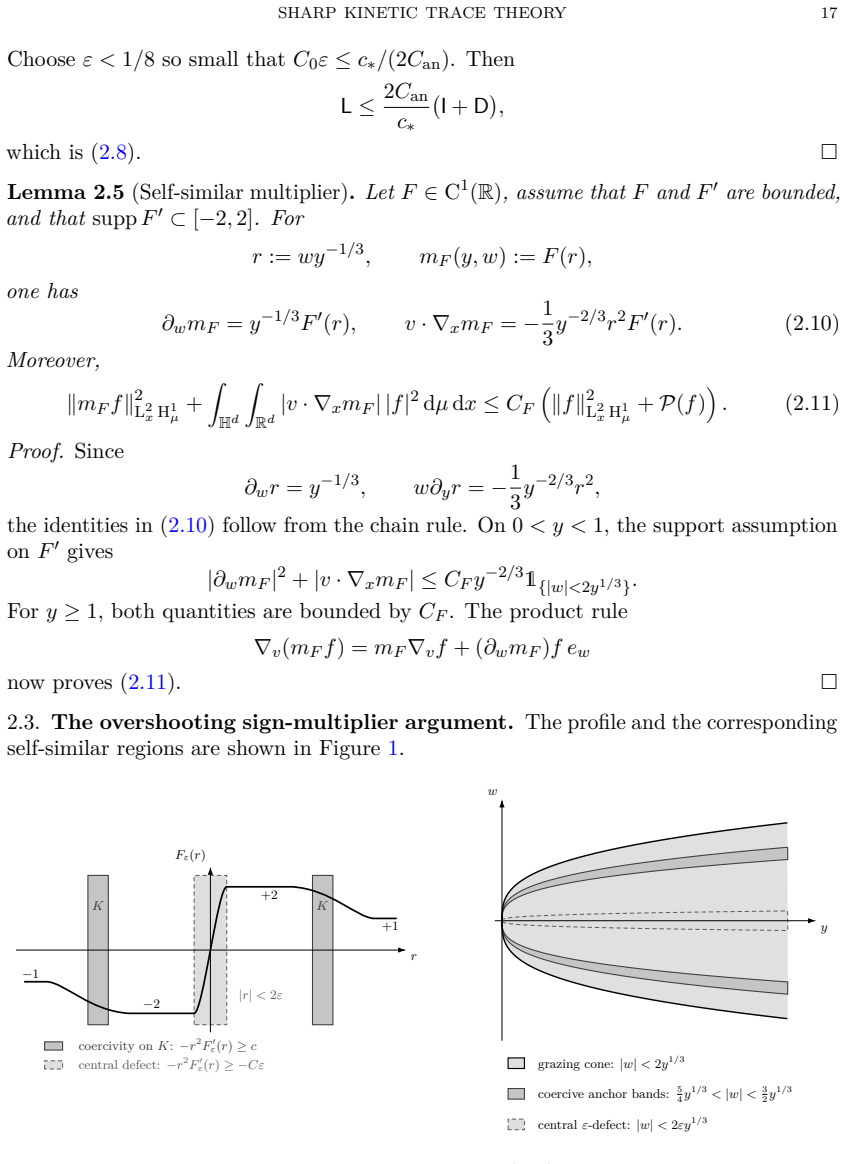
The cubic (or critical) grazing-scale multiplier: a smoothed sign profile whose transition width collapses like y^{1/3} (half-space) or like the Hölder-critical scales ρ(y)~y^{1/(p+2)}, ℓ(y)~y^{(p+1)/(p+2)} (curved domains). Combined with a one-dimensional Poincaré/Hardy transfer across the transition window, it converts Green’s identity into a boundary-flux bound while controlling the velocity-gradient cost of the multiplier.
What would settle it
On any concrete bounded C^{1,1} domain in dimension two or higher, exhibit a sequence of smooth compactly-supported test functions whose Gaussian kinetic energies stay bounded while the natural boundary integrals of |f|^2 |v·n| diverge; or, below α=1/(p+1), verify that the explicit packet family on the model domain |z|^{1+α}+|y−1|^{1+α}<1 produces a diverging ω_p boundary functional.
Extended reading notes
Core claim
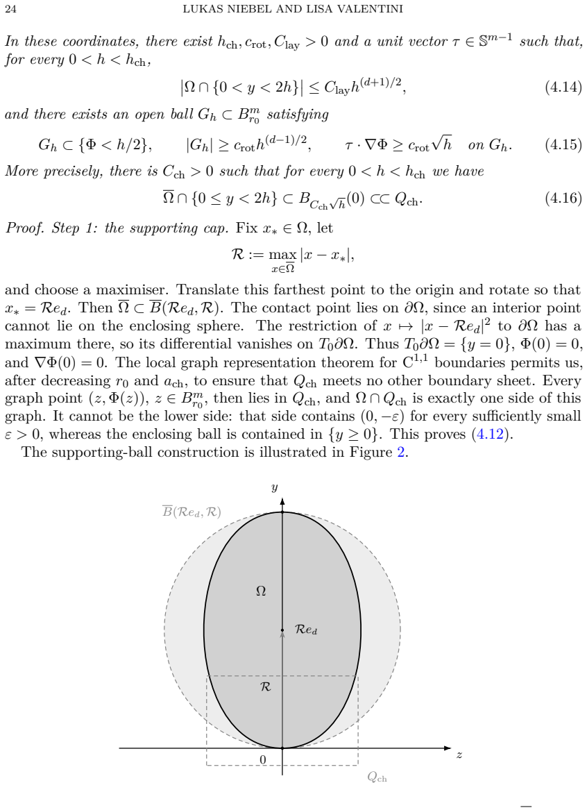
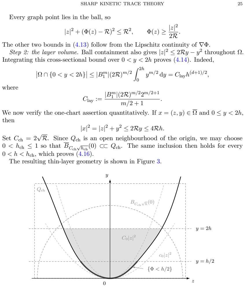
In dimensions d≥2 the natural Gaussian kinetic trace estimate fails on every bounded C^{1,1} domain, while for bounded-support Euclidean and spherical velocities the ω_p-trace estimate holds on every bounded C^{1,α} domain if and only if α≥1/(p+1), with matching existential counterexamples of exact regularity C^{1,α} below the threshold; the natural case p=1 therefore requires at least C^{1,1/2}.
Load-bearing premise
The spherical density argument for all dimensions rests on the claim that a published space–time density proof written only for dimensions two and three extends unchanged to higher dimensions by inspection.
Editorial extensions
If this is right
- Energy methods that need the natural flux weight on bounded domains must either restrict to C^{1,1/2} boundaries with bounded velocities, or accept a weaker grazing weight when velocities are unrestricted Gaussians.
- The open natural-trace question for the stationary Gaussian kinetic energy space on bounded domains is settled in the negative for d≥2.
- Green’s formula and continuous natural-trace operators are now available on half-spaces (any velocity measure) and on bounded C^{1,1/2} domains for bounded-support and spherical velocities.
- Silvestre’s quadratic grazing weight is optimal in the stationary unrestricted Gaussian setting: every weaker ω_p with p<2 fails on every C^{1,1} domain.
Reading between the lines
- Time-dependent kinetic Fokker–Planck problems on fixed cylinders inherit the same sharp exponents and regularity thresholds, because the multipliers are time-independent and the counterexamples lift by a fixed time cut-off.
- Any numerical scheme or variational formulation that relies on a natural-flux boundary term for unrestricted Gaussian velocities on a smooth bounded domain is formally unjustified and may need artificial velocity cut-offs or a weaker weight.
- The same Hölder-critical packet construction suggests that other kinetic boundary functionals (entropy fluxes, higher moments) will exhibit analogous regularity thresholds once the normal varies.
Editorial analysis
A structured set of objections, weighed in public.
Referee Report
Summary. The paper develops a comprehensive trace theory for the kinetic energy space X_μ(Ω) = {f ∈ L²(Ω;H¹_μ) : v·∇_x f ∈ L²(Ω;H^{-1}_μ)} across four velocity models. On the half-space it proves the natural (ω_1) trace estimate for unrestricted Lebesgue and Gaussian velocity measures via a cubic grazing-scale multiplier with an overshooting sign profile and a grazing-cone Hardy inequality (Theorem 2.1). On bounded C¹ domains it rules out the unrestricted Lebesgue estimate by norm-preserving velocity translation (Proposition 3.1). On every bounded C^{1,1} domain in d≥2 it proves the Gaussian ω_2 estimate (after Silvestre's multiplier) and constructs, for 1≤p<2, translated Gaussian packets on a supporting quadratic cap whose weighted boundary functional diverges like h^{(p−2)/6} while the bulk energy stays bounded (Theorem 4.2), negatively answering Question 1.8 of Albritton–Armstrong–Mourrat–Novack. For the bounded-support Euclidean and spherical models it proves the ω_p estimate on every C^{1,α} domain with α≥α_p=1/(p+1) (Theorem 6.1, Corollary 6.16) and gives matching existential counterexamples on strictly convex ℓ^q-type domains of exact regularity C^{1,α} below the threshold (Theorems 5.1–5.2). Density results then yield trace operators and Green formulas on the corresponding graph spaces (Section 7), and the one-dimensional case is classified in Section 8.
Significance. If the results hold, this is a substantial contribution to kinetic boundary theory. It resolves the natural Gaussian trace problem posed as Question 1.8 in Albritton–Armstrong–Mourrat–Novack (2024), negatively on bounded C^{1,1} domains and positively on the half-space; it identifies the sharp Hölder threshold α_p=1/(p+1) in both bounded-velocity models with matching counterexamples of exact regularity; and it proves optimality of the quadratic grazing exponent in the stationary Gaussian analogue of Silvestre's estimate. The work is constructive and falsifiable throughout: multipliers, packet families, and geometric lemmas are written out in full with explicit scales, and the paper also performs a careful audit of earlier trace claims in the literature, pinpointing where prior arguments are incomplete.
major comments (2)
- [§7.1, Proposition 7.5] Proposition 7.5 (density of C^∞(Ω×S^{d−1}) in X_σ(Ω)) is stated for all d≥2, but the proof relies on Brunken–Smetana [12, Prop. 3.1], which is stated only for d∈{2,3}. The manuscript bridges this gap with the sentence 'Inspection of its proof suggests that the same argument extends to every d≥2.' This is not a proof, and the proposition is load-bearing for the spherical trace operator of Proposition 7.9(2) and the spherical Green formula of Proposition 7.12 — both of which are claimed in the abstract ('density yields natural trace operators and Green's formula ... in the spherical velocity model'). The authors should either (a) supply the higher-dimensional argument explicitly (e.g., a short appendix verifying that the Bochner-valued spatial regularisation and the spherical H^1-basis approximation in [12, Supplement SM1] are dimension-independent), or (b) restrict Propositions 7.9(2) and
- [§1.4, Remark 1.4] Remark 1.4 asserts a full time-dependent analogue of the classification — same exponents, same thresholds, Green formulas with temporal boundary terms — with the justification 'the multiplier proofs may be rerun.' This is a substantive claim (the grazing Hardy estimate of §2 and the two-multiplier curved-boundary argument of §6 would each need a space–time Green identity and control of the ∂t terms), stated in a remark and used to conclude that 'the sharp exponents and boundary regularity thresholds in Theorem 1.1 are unchanged in the time-dependent setting.' Either a concise proof sketch indicating how the key estimates (2.15)/(6.25) absorb the temporal terms, or a softening of the claim to a conjectural remark, is needed.
minor comments (6)
- [§1.2, §2, §3, §4] Notation for test classes: throughout, C^∞_c(Ω×R^d) and C^∞_c(H^d×R^d) are used for functions that are nonzero on the spatial boundary (e.g., f_R in Prop. 3.1 is x-independent; f_h in Theorem 4.2 has χ(Φ/h)≠0; Theorem 2.1 estimates the trace at y=0 of a class that, read literally, would vanish there). The convention 'smooth functions on Ω are restrictions of ambient smooth functions' in §1.2 should be made explicit at each occurrence of the notation, since C^∞_c(H^d×R^d) taken literally would make Proposition 7.1's density statement incompatible with a nontrivial trace operator.
- [§5.2, Eq. (5.6)] Eq. (5.6): the definition of A_ℓ renders ambiguously in the text ('ℓ−m+1 2'). From the energy bound (5.11), A_ℓ² must equal ℓ^{-(m+1)}; please restore the intended exponent ℓ^{-(m+1)/2} and check the typesetting.
- [§4.2, Eq. (4.2)] Theorem 4.2: the two-sided bound T^γ_{p,Ω}(f_h) ≍ h^{(p−2)/6} is stated with subscript p,Ω on ≍ in (4.2) but the ≍ notation with subscripts is not defined; a one-line convention in §1.2 (as given for implicit constants) would help.
- [References] References [1] and [2] are the published and superseded arXiv versions of the same work. Given the careful discussion of the differences (§1.7), consider a footnote at the first citation clarifying that [2] is cited only for the historical record of the gap.
- [§4.4–4.5] In Lemma 4.5 the constant R is both the enclosing-ball radius and, later (§4.5), the packet's tangential speed R=h^{−1/3}. Although introduced in different subsections, the collision is confusing; consider renaming one of them.
- [Table 1, Figure 1] Table 1 uses 'natural for p=1' before the term 'natural trace' is used consistently in the body; a pointer to the definition after (1.6) would suffice. Figure 1's caption could state the parameter regime (0<ε<1/8 fixed by Lemma 2.4) for readability.
Circularity Check
No significant circularity: thresholds and counterexamples are derived from independent multiplier/Green identities and explicit packet constructions, not forced by definition or self-citation.
full rationale
This is a pure analysis paper whose load-bearing steps are (i) Green identities with carefully chosen multipliers (half-space cubic scale; curved-boundary height-dependent and dyadic mollified slopes), (ii) explicit finite-energy test packets (velocity translation, curvature-induced Gaussian packets, rapid-normal-variation packets on Ω_{α,d}), and (iii) density-plus-extension to obtain operators/Green formulae. The critical exponent α_p=1/(p+1) is motivated by a scaling heuristic and then confirmed by matching positive estimates and existential counterexamples; it is not fitted to data nor defined to make the claim true. Citations to Silvestre (ω_2 multiplier), Albritton–Armstrong–Mourrat–Novack (Gaussian density), and Brunken–Smetana (spherical density) supply external tools or open questions; they do not restate the paper’s sharp thresholds. The Prop. 7.5 d>3 density extension is a correctness/completeness soft spot, not a circular reduction of the claimed smooth classification or the Gaussian negative answer to Question 1.8. No self-definitional loop, fitted-as-prediction step, or load-bearing uniqueness imported from the authors’ prior work appears in the derivation chain.
Assumptions & free parameters
assumptions (6)
- standard math Classical divergence theorem / weak Gauss–Green for Lipschitz or C^1 domains and compactly supported smooth integrands, extended by density to graph spaces once traces exist.
- standard math Bounded C^{1,1} domains admit W^{1,∞} extensions of the outward normal; C^{1,α} domains admit local graph charts with α-Hölder slopes.
- domain assumption Density of compactly supported smooth functions in the unrestricted Gaussian kinetic energy space on bounded C^1 domains (Albritton–Armstrong–Mourrat–Novack Prop. 2.2).
- domain assumption Brunken–Smetana space–time smooth density on spherical-velocity graph spaces extends from d∈{2,3} to all d≥2.
- domain assumption Physical domains are at least C^1 unless a stronger hypothesis is stated; velocity measures are Lebesgue, standard Gaussian, or spherical surface measure as classified.
- standard math Odd-cancellation Gaussian primitives and Cameron–Martin unitary translations on L^2(γ) control translated packet norms (Lemmas 4.3–4.4).
invented entities (2)
-
Kinetic energy space X_μ(Ω) and weighted boundary functionals T^μ_{p,Ω} with ω_p(s)=min{s,s^p}
independent evidence
-
Cubic grazing scale a(y)=y^{1/3} and critical curved scales ρ(y)∼y^{1/(p+2)}, ℓ(y)∼y^{(p+1)/(p+2)}
independent evidence
Cite this review
Pith. "Pith review of Sharp kinetic trace theory." pith.science (2026). https://pith.science/paper/PLNIFQFF
@misc{pith2026260724708,
  author       = {Pith},
  title        = {Pith review of: Sharp kinetic trace theory},
  year         = {2026},
  howpublished = {\url{https://pith.science/paper/PLNIFQFF}},
  note         = {Machine review of arXiv:2607.24708}
}
abstract
We establish sharp kinetic trace estimates and counterexamples across several velocity models. For half-space position domains, without any common bound on velocity support, we prove the natural trace estimate for both Lebesgue and standard Gaussian velocity measures. Density yields natural trace operators and Green's formula on the corresponding kinetic energy spaces. For bounded spatial domains in $d\ge2$, in the bounded-support Euclidean velocity model and in the spherical velocity model, we identify the sharp boundary regularity threshold for the trace weights $\min\{|v \cdot n|,|v \cdot n|^p\}$, $1\le p<\infty$. Writing $\alpha_p=1/(p+1)$, the estimate holds on every bounded $\mathrm{C}^{1,\alpha}$ domain with $\alpha\ge\alpha_p$, and it fails for every $0<\alpha<\alpha_p$ on some strictly convex bounded domain of exact regularity $\mathrm{C}^{1,\alpha}$. In particular, the natural trace ($p=1$) has the regularity threshold $\mathrm{C}^{1,1/2}$. On bounded $\mathrm{C}^{1,1/2}$ domains in $d\ge2$, density yields natural trace operators and Green's formula in the bounded-support Euclidean velocity model with either Lebesgue or standard Gaussian measure, and in the spherical velocity model. Norm-preserving velocity translation rules out the unrestricted Lebesgue trace estimate on every bounded $\mathrm{C}^1$ domain. In the unrestricted Gaussian model, for each $1\le p<2$, we construct counterexamples on every bounded $\mathrm{C}^{1,1}$ domain in dimension $d\ge2$, answering Question 1.8 of Albritton, Armstrong, Mourrat, and Novack (2024) negatively. For $2\le p<\infty$, the Gaussian $\omega_2$ estimate and density instead yield $\omega_p$-trace operators.
Figures
Reference graph
Works this paper leans on
-
[1]
D. Albritton, S. Armstrong, J.-C. Mourrat, and M. Novack,Variational methods for the kinetic Fokker–Planck equation, Anal. PDE17(2024), no. 6, 1953–2010, doi:10.2140/apde.2024.17.1953
-
[2]
S. Armstrong and J.-C. Mourrat,Variational methods for the kinetic Fokker–Planck equation, arXiv:1902.04037v1 (2019),https://arxiv.org/abs/1902.04037v1
arXiv 1902
-
[3]
P. Auscher, C. Imbert, and L. Niebel,Weak solutions to Kolmogorov–Fokker–Planck equations: regularity, existence and uniqueness, arXiv:2403.17464 (2024)
arXiv 2024
- [4]
-
[5]
B. Avelin and M. Hou,Weak and Perron solutions for stationary Kramers–Fokker–Planck equations in bounded domains, Potential Anal.64(2026), Article 11, doi:10.1007/s11118-025-10242-z
-
[6]
G. Bal and B. Palacios,Pencil-beam approximation of stationary Fokker–Planck, SIAM J. Math. Anal.52(2020), no. 4, 3487–3519, doi:10.1137/19M1295775
-
[7]
M. S. Baouendi and P. Grisvard,Sur une équation d’évolution changeant de type, J. Funct. Anal.2 (1968), 352–367, doi:10.1016/0022-1236(68)90012-8. SHARP KINETIC TRACE THEORY 61
-
[8]
C. Bardos,Problèmes aux limites pour les équations aux dérivées partielles du premier ordre à coefficients réels; théorèmes d’approximation; application à l’équation de transport, Ann. Sci. École Norm. Sup. (4)3(1970), 185–233, doi:10.24033/asens.1190
Show all 38 references
-
[9]
Bernard,On the existence and asymptotic behavior of weak solution of the kinetic Fokker–Planck equation in a bounded domain with absorbing boundary, Bull
É. Bernard,On the existence and asymptotic behavior of weak solution of the kinetic Fokker–Planck equation in a bounded domain with absorbing boundary, Bull. Sci. Math.197(2024), Paper No. 103523, doi:10.1016/j.bulsci.2024.103523
2024
-
[10]
Bosboom, H
V. Bosboom, H. Egger, and M. Schlottbom,Analysis and systematic discretization of a Fokker– Planck equation with Lorentz force, Comput. Methods Appl. Math.25(2025), no. 4, 807–822, doi:10.1515/cmam-2025-0061
2025 doi
-
[11]
Boyer,Trace theorems and spatial continuity properties for the solutions of the transport equation, Differential Integral Equations18(2005), no
F. Boyer,Trace theorems and spatial continuity properties for the solutions of the transport equation, Differential Integral Equations18(2005), no. 8, 891–934, doi:10.57262/die/1356060150
2005
-
[12]
Brunken and K
J. Brunken and K. Smetana,Stable and efficient Petrov–Galerkin methods for a kinetic Fokker–Planck equation, SIAM J. Numer. Anal.60(2022), no. 1, 157–179, doi:10.1137/20M1374857
2022 doi
-
[13]
Cannone and C
M. Cannone and C. Cercignani,A trace theorem in kinetic theory, Appl. Math. Lett.4(1991), no. 6, 63–67, doi:10.1016/0893-9659(91)90077-9
1991 doi
-
[14]
Carrapatoso, P
K. Carrapatoso, P. Gabriel, R. Medina, and S. Mischler,Constructive Krein–Rutman result for kinetic Fokker–Planck equations in a domain, arXiv:2407.10530 (2024)
2024 arXiv
-
[15]
Carrapatoso and S
K. Carrapatoso and S. Mischler,The kinetic Fokker–Planck equation in a domain: ultracontractivity, hypocoercivity, and long-time asymptotic behavior, Rend. Lincei Mat. Appl.35(2024), no. 4, 643–680, doi:10.4171/RLM/1055
2024 doi
-
[16]
J. A. Carrillo,Global weak solutions for the initial-boundary-value problems to the Vlasov–Poisson– Fokker–Planck system, Math. Methods Appl. Sci.21(1998), no. 10, 907–938,doi:10.1002/(SICI) 1099-1476(19980710)21:10<907::AID-MMA977>3.0.CO;2-W
1998 doi
-
[17]
Cessenat,Théorèmes de traceLp pour des espaces de fonctions de la neutronique, C
M. Cessenat,Théorèmes de traceLp pour des espaces de fonctions de la neutronique, C. R. Acad. Sci. Paris Sér. I Math.299(1984), no. 16, 831–834
1984
-
[18]
Cessenat,Théorèmes de trace pour des espaces de fonctions de la neutronique, C
M. Cessenat,Théorèmes de trace pour des espaces de fonctions de la neutronique, C. R. Acad. Sci. Paris Sér. I Math.300(1985), no. 3, 89–92
1985
-
[19]
Choi and S
Y.-P. Choi and S. Song,Global weak solutions to nonlinear kinetic Fokker–Planck equations in bounded domains under physical initial data, arXiv:2510.06656 (2025)
2025
-
[20]
Degond and S
P. Degond and S. Mas–Gallic,Existence of solutions and diffusion approximation for a model Fokker–Planck equation, Transport Theory Statist. Phys.16(1987), nos. 4–6, 589–636, doi:10.1080/00411458708204307
1987 doi
-
[21]
Garain and K
P. Garain and K. Nyström,On regularity and existence of weak solutions to nonlinear Kolmogorov– Fokker–Planck type equations with rough coefficients, Math. Eng.5(2023), no. 2, 1–37, doi:10.3934/mine.2023043
2023 doi
-
[22]
Y. Guo, C. Kim, D. Tonon, and A. Trescases,Regularity of the Boltzmann equation in convex domains, Invent. Math.207(2017), no. 1, 115–290, doi:10.1007/s00222-016-0670-8
2017 doi
-
[23]
Henderson, G
C. Henderson, G. Lucertini, and W. Wang,A kinetic Nash inequality and precise boundary behavior of the kinetic Fokker–Planck equation, arXiv:2407.08785 (2024)
2024 arXiv
-
[24]
Hou,Boundedness of weak solutions to degenerate Kolmogorov equations of hypoel- liptic type in bounded domains, J
M. Hou,Boundedness of weak solutions to degenerate Kolmogorov equations of hypoel- liptic type in bounded domains, J. Differential Equations453(2026), Paper No. 113794, doi:10.1016/j.jde.2025.113794
2026
-
[25]
H. J. Hwang, J. Jang, and J. J. L. Velázquez,The Fokker–Planck equation with absorbing boundary conditions, Arch. Ration. Mech. Anal.214(2014), no. 1, 183–233, doi:10.1007/s00205-014-0758-5
2014 doi
-
[26]
Kim and M
K. Kim and M. Weidner,Sharp regularity near the grazing set for kinetic Fokker–Planck equations, arXiv:2603.04121 (2026)
2026
-
[27]
Kim and M
K. Kim and M. Weidner,Kinetic Fokker–Planck equations with Maxwell boundary conditions, arXiv:2607.20076 (2026)
2026 arXiv
-
[28]
Litsgård and K
M. Litsgård and K. Nyström,The Dirichlet problem for Kolmogorov–Fokker–Planck type equations with rough coefficients, J. Funct. Anal.281(2021), no. 10, Paper No. 109226, doi:10.1016/j.jfa.2021.109226
2021
-
[29]
T. A. Manteuffel, K. J. Ressel, and G. Starke,A boundary functional for the least-squares finite- element solution of neutron transport problems, SIAM J. Numer. Anal.37(2000), no. 2, 556–586, doi:10.1137/S0036142998344706. 62 LUKAS NIEBEL AND LISA V ALENTINI
2000 doi
-
[30]
E. J. McShane,Extension of range of functions, Bull. Amer. Math. Soc.40(1934), no. 12, 837–842, doi:10.1090/S0002-9904-1934-05978-0
1934 doi
-
[31]
Mischler,On the trace problem for solutions of the Vlasov equation, Comm
S. Mischler,On the trace problem for solutions of the Vlasov equation, Comm. Partial Differential Equations25(2000), no. 7–8, 1415–1443, doi:10.1080/03605300008821554
2000 doi
-
[32]
Mischler,Kinetic equations with Maxwell boundary conditions, Ann
S. Mischler,Kinetic equations with Maxwell boundary conditions, Ann. Sci. École Norm. Sup. (4)43 (2010), no. 5, 719–760, doi:10.24033/asens.2132
2010 doi
-
[33]
Nier,Boundary conditions and subelliptic estimates for geometric Kramers–Fokker–Planck op- erators on manifolds with boundaries, Mem
F. Nier,Boundary conditions and subelliptic estimates for geometric Kramers–Fokker–Planck op- erators on manifolds with boundaries, Mem. Amer. Math. Soc.252(2018), no. 1200, v+144 pp., doi:10.1090/memo/1200
2018 doi
-
[34]
Ouyang and L
Z. Ouyang and L. Silvestre,ConditionalL∞ estimates for the non-cutoff Boltzmann equation in a bounded domain, Arch. Ration. Mech. Anal.248(2024), no. 4, Paper No. 59, doi:10.1007/s00205- 024-02002-x
2024 doi
-
[35]
Ros-Oton and M
X. Ros-Oton and M. Weidner,Optimal regularity for kinetic Fokker–Planck equations in domains, arXiv:2505.11943 (2025)
2025 arXiv
-
[36]
Silvestre,Hölder estimates for kinetic Fokker–Planck equations up to the boundary, Ars Inven
L. Silvestre,Hölder estimates for kinetic Fokker–Planck equations up to the boundary, Ars Inven. Anal. (2022), Paper No. 6, 29 pp., doi:10.15781/nqdd-qs03
2022 doi
-
[37]
Valentini,Well-posedness and trace theory for the Kolmogorov equation on bounded domains, arXiv:2606.19198 (2026)
L. Valentini,Well-posedness and trace theory for the Kolmogorov equation on bounded domains, arXiv:2606.19198 (2026)
2026 arXiv
-
[38]
Zhu,Regularity of kinetic Fokker–Planck equations in bounded domains, Ann
Y. Zhu,Regularity of kinetic Fokker–Planck equations in bounded domains, Ann. Henri Lebesgue7 (2024), 1323–1366, doi:10.5802/ahl.221. (Lukas Niebel)Institut für Analysis und Numerik, Universität Münster, Orléans-Ring 10, 48149 Münster, Germany. Email address:lukas.niebel@uni-m...
2024 doi
Reviewed July 31, 2026 · model on record in the stance chip above.
Discussion (0). Continue with ORCID to comment.