Prediction of experimental excited-state absorption spectra by using vibronic transition calculations: Its practical application to a {\pi}-conjugated molecule

Joonyoung F. Joung; Sungnam Park

REVIEW 1 major objections 4 minor 60 references

Prediction of experimental excited-state absorption spectra by using vibronic transition calculations: Its practical application to a {\pi}-conjugated molecule

T0 review · 1 major / 4 minor · reviewed 2026-08-01 · deepseek-v4-flash

Challenge this review Re-run · record.json Download PDF Read on arXiv ↗

Pith's one-line read Vibronic transition calculations reproduce azulene's excited-state absorption bands and reassign several peaks.

desk verdict Practical and honest for band shapes, but the fitted energy corrections mean the 'predicted' ESA positions are partly calibrated to the same data; the real product is a quick assignment tool, not independent prediction. read the letter →

arxiv 2607.25247 v1 pith:JYCDUTNC submitted 2026-07-28 cs.CE

Joonyoung F. Joung , Sungnam Park This is my paper · ORCID

classification cs.CE

keywords excited-stateabsorptionvibronictransitionFranck-CondonHerzberg-TellerTDDFTazulenetransientbandassignment

verification ladder T0 review T1 audit T2 compute T3 formal

The pith

A machine-rendered reading of the paper's core claim, the machinery that carries it, and where it could break.

The reading

The paper tries to establish that excited-state absorption (ESA) spectra can be predicted practically by combining vibronic (Franck-Condon) transition calculations with routine density functional theory, without needing excited-state-to-excited-state transition moments. Using azulene as a test case, the method reproduces the vibronic band shapes and peak positions of the experimental transient-absorption spectrum, and it reassigns several ESA peaks to different electronic transitions than earlier multireference calculations suggested. If true, this gives experimentalists a straightforward way to assign ESA bands in transient and photoinduced absorption spectra using standard quantum-chemistry packages.

What carries the argument

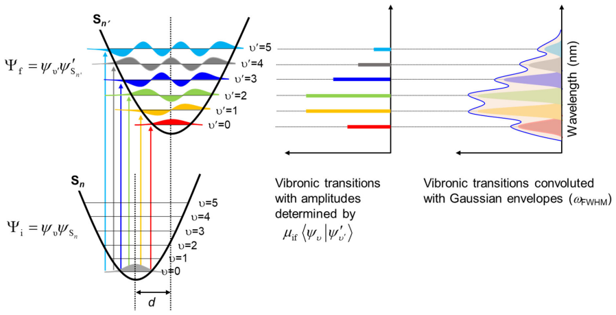
The central object is the Franck-Condon–Herzberg-Teller vibronic transition calculation (adiabatic Hessian, time-independent framework at 298 K) between two electronic states, which yields the vibrational band shape from the overlap of harmonic vibrational wavefunctions. Its inputs are the pair of potential energy surfaces obtained from DFT/TDDFT frequency calculations. To compare with experiment, the calculation uses an empirical energy correction σ_ESA = σ(S0→Sn′) − σ(S0→Sn) and approximates the ESA line width as the sum of the two ground-state transition line widths.

What would settle it

Compute the S1→S4 transition energy of azulene with a wavefunction method that includes explicit excited-to-excited transition moments; if that energy lies outside the observed ESA band near 375 nm and its computed vibronic progression does not match the measured band shape, the central assignment fails.

Watch

Extended reading notes

Core claim

The paper shows that the vibronic band shapes and peak positions of ESA spectra can be obtained from Franck-Condon–Herzberg-Teller vibronic transition calculations between two electronic states, using only the potential energy surfaces (equilibrium geometry, vibrational frequencies, normal modes) that routine DFT/TDDFT provides. Because Franck-Condon factors depend only on the potential energy surfaces and not on the electronic transition moment between the two excited states, the method circumvents the need for excited-to-excited transition moments. For azulene, the calculated ESA bands reproduce the experimental transient-absorption spectrum and lead to different assignments than earlier m

Load-bearing premise

The predicted ESA band positions rest on an empirical rule that sets the excited-state energy correction as the difference of two fitted ground-state corrections (σ_ESA = σ_S0→Sn′ − σ_S0→Sn); if the TDDFT systematic error does not cancel in that difference, every predicted ESA peak shifts coherently and the assignments fail.

Editorial extensions

If this is right

ESA bands in transient absorption and photoinduced absorption spectra of molecules with well-behaved excited-state potential energy surfaces can be assigned to specific electronic transitions using only standard DFT/TDDFT calculations.
Transitions whose surrogate S0→Sn′ transition has zero oscillator strength are invisible in this scheme even if the actual excited-state transition is allowed, as with S1→S5 in azulene.
Vibronic calculations identify the vibrational normal modes coupled to each electronic transition, directly pointing to the modes that drive excited-state structural changes.
The method is restricted to band positions and shapes; absolute ESA intensities still require quadratic-response or explicit excited-to-excited transition-moment evaluations.
The azulene reassignments imply that matching vibronic band shapes, not just vertical transition energies, is a useful criterion for assigning ESA bands.

Reading between the lines

Editorial extensions of the paper, not claims the author makes directly.

If the empirical subtraction rule for the energy correction transfers TDDFT's systematic error, the approach should generalize to other π-conjugated molecules; a natural test is to apply it to molecules with known ESA spectra and compare the assigned transitions.
The azulene reassignments suggest some published ESA assignments based on vertical excitation energies alone may be worth revisiting with band-shape information.
The harmonic treatment of azulene's bent S4 state is explicitly approximate; for such double-well surfaces, an anharmonic or multireference treatment would be needed, and band-shape predictions there should be treated as qualitative.
Combining the calculated vibronic band shapes with measured ESA intensities could provide a route to estimate excited-to-excited transition moments by intensity fitting.

Share X Bluesky LinkedIn Reddit HN

Editorial analysis

A structured set of objections, weighed in public.

Desk editor's note, referee report, and a circularity audit.

Desk Editor's Note

read the letter

First things first: the core idea is that vibronic band shapes for excited-state absorption can be computed from PESs alone, using ordinary TDDFT frequency calculations, without needing excited-to-excited transition moments. That is a useful and honest simplification. The authors apply it to azulene and obtain band shapes that resemble the experimental transient absorption, and they offer new assignments for the 375 nm and 575 nm ESA features. The writing is clear and the limitations are stated up front.

What is genuinely new: Gierschner and co-workers had already demonstrated the vibronic approach with QR-TDDFT. This paper shows that routine TDDFT (APFD, etc.) may suffice, and it identifies specific coupled modes. The azulene absorption/emission benchmarks look good, giving some confidence that the PESs are reasonable.

The soft spot is the energy-scale correction. The authors fit a sigma to each S0→Sn transition to match experiment, then set the ESA shift to the difference of two sigmas. That assumes the TDDFT error for the initial and final excited states cancels. A careful reader will see this is load-bearing and unvalidated; if the cancellation fails by 0.1 eV, the reassignments become shaky. The paper does not discuss this transfer rule. The missing SI tables also prevent me from checking fitted values or doing replication.

Second, the S4 state is anharmonic (double well), and the harmonic adiabatic-Hessian treatment is acknowledged to be approximate. That is one of the two main new assignments (S1→S4), so the claim should be softer. The intensities are not predicted, and the 1/13 scaling is just for visualization; fine, but it means validation is by eye.

Third, the abstract says the method 'reproduces the vibronic features and band positions.' That overstates it, since the band positions are adjusted by the fit. The band shapes are the genuine product.

Overall: this is a serious, useful contribution for practitioners who want a quick way to assign ESA bands. It deserves a proper referee, but the authors should address the sigma transfer rule (e.g., test on a few molecules with known assignments or report sensitivity), include the SI data, and soften the position-claim. I would cite it if the SI and the revised argument hold up.

Recommendation: send to peer review, with major revision.

Referee Report

1 major / 4 minor

Summary. The paper proposes a practical methodology for predicting excited-state absorption (ESA) spectra by combining standard TDDFT geometry and frequency calculations with vibronic transition (Franck–Condon/Herzberg–Teller) calculations. Using azulene as a test system, the authors compute S1→Sn and S2→Sn vibronic band shapes and peak positions, compare them with transient absorption spectra, and reassign several ESA features (e.g., 375 nm to S1→S4, 575 nm to S2→S8/S9 instead of S2→S11). Absolute ESA intensities are not predicted; instead, a correction rule (σ_ESA = σ_S0→Sn' − σ_S0→Sn) and additive Gaussian widths are used, with the electronic transition moment taken from the corresponding S0→Sn' transition. The paper is explicitly framed as a practical, accessible alternative to specialized quadratic-response or real-time TDDFT methods.

Significance. If the central claim holds, the method would be valuable for interpreting transient-absorption and photoinduced-absorption spectra using only routine Gaussian 16 calculations, without requiring excited-to-excited transition moments. The paper is honest about its limitations: it acknowledges the harmonic approximation failure for the S4 state, the neglect of absolute intensities, and the approximate nature of the linewidth combination rule. The strengths are the transparency of the approach, the use of a well-studied molecule, and the direct identification of coupled normal modes. However, because the predicted ESA peak positions inherit a fitted correction that is not independently validated, and because one of the two main new assignments involves a state admitted to be anharmonic, the practical usefulness for band assignment is currently demonstrated only qualitatively and conditionally.

major comments (1)

[Section 3.3] The comparison between calculated and experimental ESA spectra is entirely visual and uses an arbitrary scaling factor (1/13 in Figure 4b) for the key S1→S4 transition. Given that the central claim is that the method 'reproduces the vibrational band shapes and positions,' the absence of any quantitative metric (e.g., root-mean-square difference in peak positions, spectral overlap integral, or at least a table of calculated vs. experimental peak maxima for all assigned features) makes it impossible to judge how good the agreement actually is. The ω_FWHM values (800 cm⁻¹ in Figure 3, 2000 cm⁻¹ in Figure 4) are chosen ad hoc; their effect on the apparent agreement should be discussed, and the sensitivity of the assignments to these widths should be assessed.

minor comments (4)

[Section 2] The sentence 'Consequently, the present scheme does not provide absolute or relative ESA intensities' is repeated almost verbatim in Section 4; one occurrence could be removed. The notation in Eq. (5) is unclear: S is called 'the calculated spectrum' but is later convoluted with a Gaussian; it might be clearer to denote the stick spectrum explicitly.
[Figure 4 caption] The caption says 'ω_FWHM = 2000 cm⁻¹ in (a) and (c)', but those panels are experimental spectra; presumably the experimental spectra are shown as measured and ω_FWHM applies to the calculated spectra in (b) and (d). This needs clarification.
[References] Reference 44 has a typo: 'ull. Korean Chem. Soc.' should be 'Bull. Korean Chem. Soc.' Also, reference 42 (Gaussian 16) is cited in a nonstandard format; consistent citation of the software manual would be preferable.
[Section 3.2] The sentence 'as can be evinced from the data reported in Figure 4(b)' appears twice in consecutive paragraphs; one can be removed. The phrase 'this does not imply that the S1→S5 and S2→S5 transitions are themselves forbidden' is good but could be accompanied by a short explanation of why the approximation fails for S5 rather than just stating it.

Circularity Check

1 steps flagged · score 6.0 of 10

ESA peak positions are anchored to fitted S0→Sn corrections: σ_ESA = σ(S0→Sn′) − σ(S0→Sn) makes the corrected ESA electronic energy equal to the difference of the experimental absorption peaks used for calibration, so only vibronic band shapes are genuinely independent.

fitted input called prediction [Section 2, after Eq. (5); applied in Section 3.2, Figure 4(b,d)]
"The Gaussian envelopes (ωFWHM) and correction factors for the absorption and emission transitions were determined by comparing them with the corresponding experimentally measured absorption and emission peaks... The value of σ of the ESA transition (Sn→Sn′) was approximately determined by calculating the difference of the two σ values for the S0→Sn and S0→Sn′ transitions."

Let C_n be the calculated S0→Sn peak and E_n its experimental counterpart. Fitting defines σ_n = E_n − C_n. The ESA correction is σ_n′ − σ_n, so the corrected ESA peak is (C_n′ − C_n) + (E_n′ − C_n′) − (E_n − C_n) = E_n′ − E_n, up to a Franck–Condon shift difference between the ESA band and the two S0→Sn bands. Thus the TDDFT electronic energies cancel identically; the reported ESA band positions are not independent predictions but a rearrangement of the experimental S0→Sn absorption peak differences used for calibration. The genuinely computed content is the vibronic band shape and the differential FC shift, not the absolute electronic energy of the ESA transition.

full rationale

The method is not wholly circular: vibronic band shapes are computed from TDDFT potential-energy surfaces and are not fitted to ESA data; the assignment of specific Sn→Sn′ transitions is nontrivial; and the 1/13 intensity scaling is explicitly presented as a non-predictive normalization. The paper's self-citations are to the authors' earlier photophysics work and are not load-bearing for the method; no uniqueness theorem is invoked and no ansatz is smuggled in via citation. The significant circular step is the ESA position correction: σ_ESA is defined as the difference of per-state σ values fitted to experimental S0→Sn peaks, which algebraically cancels the calculated excited-state electronic energy difference and anchors the ESA peak position to experimental absorption peak differences. Consequently, the 'positions' part of the central claim ('reproduce the vibrational band shapes and positions of the ESA features') reduces by construction to the calibration data, while the 'shapes' part remains independent. The acknowledged limitations—harmonic approximation failing for S4 and the lack of excited-to-excited transition moments—are correctness risks rather than circularity. Score 6 reflects partial, not total, circularity: the energy scale of the predicted ESA bands is imposed by the fitted inputs, but the vibronic structure and state assignments retain independent computational content.

Assumptions & free parameters 3 free parameters · 5 assumptions · 0 invented entities

The method adds no new physical entities. It relies on standard vibronic theory and a set of fitted correction parameters.

free parameters (3)

σ (correction factor) for S0→Sn transitions = not listed (Table S1 absent)
Shift computed transition energies to match experimental absorption/emission peaks; used in Eq. (5) and combined for ESA via σ_ESA = σ_S0→Sn' − σ_S0→Sn.
ω_FWHM (Gaussian linewidth) for absorption/emission = e.g., 300 cm⁻¹ for S0→Sn; ESA 800–2000 cm⁻¹
Chosen to match experimental line shapes; ESA width approximated as sum of the two S0→Sn widths.
intensity scaling factor for S1→S4 ESA = 1/13
Arbitrary scaling to overlay calculated band shape with experimental ESA spectrum in Fig. 4(b).

assumptions (5)

standard math Born-Oppenheimer separation of electronic and nuclear wavefunctions
Invoked in Section 2 (Eq. 2) to factor transition dipole into electronic and vibrational parts.
standard math Franck-Condon and Herzberg-Teller expansions of the transition moment
Eqs. (3)-(4) in Section 2; standard treatment but requires PESs and normal modes.
domain assumption Harmonic approximation for excited-state potential energy surfaces
Used in adiabatic-Hessian vibronic calculation; Section 3.3 admits S4 is bent/anharmonic, so harmonic description is approximate.
domain assumption Excited-to-excited transition moment approximated by S0→Sn′ transition moment
Section 2: 'the moment used here for an Sn→Sn′ transition is that of the corresponding S0→Sn′ transition'; allows band-shape calculation but prevents intensity prediction.
ad hoc to paper Additivity of FWHM and difference rule for σ when constructing ESA spectra
Section 2: ESA ω_FWHM = sum of two S0→Sn widths; σ_ESA = difference of two σ values. No independent justification; authors note it may fail for charge-separated states.

how reviews work

0 comments

Cite this review

Pith. "Pith review of Prediction of experimental excited-state absorption spectra by using vibronic transition calculations: Its practical application to a {\pi}-conjugated molecule." pith.science (2026). https://pith.science/paper/JYCDUTNC

@misc{pith2026260725247,
  author       = {Pith},
  title        = {Pith review of: Prediction of experimental excited-state absorption spectra by using vibronic transition calculations: Its practical application to a \pi-conjugated molecule},
  year         = {2026},
  howpublished = {\url{https://pith.science/paper/JYCDUTNC}},
  note         = {Machine review of arXiv:2607.25247}
}

read the original abstract

Accurate theoretical prediction of excited-state absorption (ESA) spectra remains challenging. Although considerable progress has been made in computational methods for ESA spectroscopy, their practical application to the interpretation of transient absorption and photoinduced absorption spectra is still limited. In this study, we present a practical approach for calculating molecular ESA spectra by combining vibronic transition calculations with routine density functional theory (DFT) and time-dependent DFT (TDDFT) calculations available in standard quantum chemistry packages. Using azulene as a model system, we demonstrate that the proposed method successfully reproduces the vibronic features and band positions observed in the experimental ESA spectrum. This approach therefore provides a practical framework for assigning ESA bands arising from transitions between low-lying excited states of molecules. The method delivers the vibronic band shapes and peak positions that are needed to assign ESA bands directly from these standard calculations, without requiring the excited-state-to-excited-state transition moments that determine absolute intensities.

Figures

Figures reproduced from arXiv: 2607.25247 by the authors.

**Figure 1.** Schematic of the calculation of the vibronic transitions (SnSn). The molecular geometry optimization, vibrational frequencies, and vibronic spectra were obtained by applying the DFT45 and TDDFT46-49 methods at the APFD,50 B3LYP,51 CAMB3LYP,52 and B97XD53 levels with a 6-311++G(d,p) basis set,54 as implemented in the Gaussian 16 package.42 The vibronic transition calculations were carried out by using FranckCond… view at source ↗

Discussion (0). Continue with ORCID to comment.

Reference graph

Works this paper leans on

60 extracted references

[1]

S. Kim, S. Lee, T. F. Anjong, H. Y . Jang, J.-Y . Kim, C. Lee, S. Park, H. J. Lee, J. Yoon, J. Kim, J. Phys. Chem. C 2016, 120, 28407-28414

2016
[2]

Kafizas, X

A. Kafizas, X. Wang, S. R. Pendlebury, P. Barnes, M. Ling, C. Sotelo-Vazquez, R. Quesada-Cabrera, C. Li, I. P. Parkin, J. R. Durrant, J. Phys. Chem. A 2016, 120, 715- 723

2016
[3]

Zirzlmeier, D

J. Zirzlmeier, D. Lehnherr, P. B. Coto, E. T. Chernick, R. Casillas, B. S. Basel, M. Thoss, R. R. Tykwinski, D. M. Guldi, Proc. Natl. Acad. Sci. U.S.A. 2015, 112, 5325-5330

2015
[4]

J. F. Joung, S. Kim, S. Park, J Phys Chem B 2015, 119, 15509-15515

2015
[5]

J. F. Joung, S. Kim, S. Park, Phys. Chem. Chem. Phys. 2017, 19, 25509-25517

2017
[6]

J. F. Joung, S. Kim, S. Park, J Phys Chem B 2018, 122, 5087-5093

2018
[7]

Y . Hu, J. F. Joung, J.-E. Jeong, Y . Jeong, H. Y . Woo, Y . She, S. Park, J. Yoon, Sens. Actuators B 2019, 280, 298-305

2019
[8]

Ravi Kumar, F

V . Ravi Kumar, F. Ariese, S. Umapathy, J. Chem. Phys. 2016, 144, 114301

2016

Show all 60 references

[9]

Quick, A

M. Quick, A. L. Dobryakov, I. N. Ioffe, F. Berndt, R. Mahrwald, N. P. Ernsting, S. A. Kovalenko, J Phys Chem B 2018, 122, 1049-1059

2018
[10]

S. He, P. Jin, T. Lian, H. Zhu, Nat. Rev. Methods Primers 2026, 6, 34

2026
[11]

Santoro, R

F. Santoro, R. Improta, A. Lami, J. Bloino, V . Barone, J. Chem. Phys. 2007, 126, 084509

2007
[12]

Santoro, A

F. Santoro, A. Lami, R. Improta, V . Barone, J. Chem. Phys. 2007, 126, 184102

2007
[13]

Barone, J

V . Barone, J. Bloino, M. Biczysko, F. Santoro, J. Chem. Theory Comput. 2009, 5, 540- 554

2009
[14]

Baiardi, J

A. Baiardi, J. Bloino, V . Barone, J. Chem. Theory Comput. 2013, 9, 4097-4115

2013
[15]

de Jong, L

M. de Jong, L. Seijo, A. Meijerink, F. T. Rabouw, Phys. Chem. Chem. Phys. 2015, 17, 16959-16969

2015
[16]

Bloino, A

J. Bloino, A. Baiardi, M. Biczysko, Int. J. Quantum Chem. 2016, 116, 1543-1574

2016
[17]

Sirucek, B

J. Sirucek, B. Le Guennic, Y . Damour, P.-F. Loos, D. Jacquemin, J. Chem. Theory Comput. 2025, 21, 4688-4703

2025
[18]

D. A. Fedotov, A. C. Paul, P. Posocco, F. Sa ntoro, M. Garavelli, H. Koch, S. Coriani, R. Improta, J. Chem. Theory Comput. 2021, 17, 1638-1652

2021
[19]

Petersilka, U

M. Petersilka, U. J. Gossmann, E. K. Gross, Phys. Rev. Lett. 1996, 76, 1212-1215

1996
[20]

Zangwill, P

A. Zangwill, P. Soven, Phys Rev A 1980, 21, 1561-1572

1980
[21]

Bauernschmitt, R

R. Bauernschmitt, R. Ahlrichs, Chem. Phys. Lett. 1996, 256, 454-464

1996
[22]

A. J. Thorvaldsen, K. Ruud, K. Kristensen, P. Jorgensen, S. Coriani, J. Chem. Phys. 2008, 129, 214108. 20

2008
[23]

Runge, E

E. Runge, E. K. U. Gross, Phys. Rev. Lett. 1984, 52, 997-1000

1984
[24]

F. Aiga, T. Tada, R. Yoshimura, J. Chem. Phys. 1999, 111, 2878-2888

1999
[25]

S. M. Parker, S. Roy, F. Furche, J. Chem. Phys. 2016, 145, 134105

2016
[26]

D. Jeon, K. C. Cho, Y . K. Kang, Bull. Korean Chem. Soc. 2025, 46, 281-292

2025
[27]

M. A. Mosquera, L. X. Chen , M. A. Ratner, G. C. Schatz, J. Chem. Phys. 2016, 144, 204105

2016
[28]

M. A. Mosquera, N. E. Jackson, T. J. Fauve ll, M. S. Kelley, L. X. Chen, G. C. Schatz, M. A. Ratner, J. Am. Chem. Soc. 2017, 139, 3728-3735

2017
[29]

E. F. Oliveira, J. Shi, F. C. Lavarda, L. Luer, B. Milian-Medina, J. Gierschner, J. Chem. Phys. 2017, 147, 034903

2017
[30]

S. M. Parker, D. Rappoport, F. Furche, J. Chem. Theory Comput. 2018, 14, 807-819

2018
[31]

S. A. Fischer, C. J. Cramer, N. Govind, J. Chem. Theory Comput. 2015, 11, 4294-4303

2015
[32]

S. A. Fischer, C. J. Cramer, N. Govind, J. Phys. Chem. Lett. 2016, 7, 1387-1391

2016
[33]

D. N. Bowman, J. C. Asher, S. A. Fischer, C. J. Cramer, N. Govind, Phys. Chem. Chem. Phys. 2017, 19, 27452-27462

2017
[34]

Lopata, N

K. Lopata, N. Govind, J. Chem. Theory Comput. 2011, 7, 1344-1355

2011
[35]

Mehmood, M

A. Mehmood, M. C. Silfies, A. S. Durden, T. K. Allison, B. G. Levine, J. Chem. Phys. 2024, 161

2024
[36]

Perez-Castillo, V

R. Perez-Castillo, V . M. Freixas, S. Muka mel, A. Martinez-Mesa, L. Uranga-Piña, S. Tretiak, M. F. Gelin, S. Fernandez-Alberti, Chem. Sci. 2024, 15, 13250-13261

2024
[37]

W. Park, S. Lee, K. Komarov, V . Mironov, H. Nakata, T. Zeng, M. Huix ‐Rotllant, C. H. Choi, Bull. Korean Chem. Soc. 2025, 46, 330-346

2025
[38]

A. Lami, C. Petrongolo, F. Santoro, in Conical Intersections (Ed.: W. Domcke, Yarkony, R., Koeppel, H.), World Scientific Publishing Co., Singapore, 2004, pp. 699-738

2004
[39]

P. T. Ruhoff, Chem. Phys. 1994, 186, 355-374

1994
[40]

T. Lu, F. Chen, J. Comput. Chem. 2012, 33, 580-592

2012
[41]

Sarkar, M

R. Sarkar, M. Boggio-Pasqua, P.-F. Loos, D. Jacquemin, J. Chem. Theory Comput. 2021, 17, 1117-1132

2021
[42]

G. W. T. M. J. Frisch, H. B. Schlegel, G. E. Scuseria, M. A. Robb, J. R. Cheeseman, G. Scalmani, V . Barone, G. A. Petersson, H. Nakatsuji, X. Li, M. Caricato, A. V . Marenich, J. Bloino, B. G. Janesko, R. Gomperts, B. Mennucci, H. P. Hratchian, J. V . Ortiz, A. F. Izmaylov, J...

2016
[43]

X. Wu, X. Xie, A. Troisi, J. Mater. Chem. C 2024, 12, 18886-18892

2024
[44]

Kupriyanova, B

L. Kupriyanova, B. F. Soeriawidjaja, J. Hwang, M. Park, M. Kwak, Y. Kim, ull. Korean Chem. Soc. 2025, 46, 526-539

2025
[45]

J. A. Pople, P. M. W. Gill, B. G. Johnson, Chem. Phys. Lett. 1992, 199, 557-560

1992
[46]

M. E. Casida, C. Jamorski, K. C. Casida, D. R. Salahub, J. Chem. Phys. 1998, 108, 4439-4449

1998
[47]

J. Liu, W. Liang, J. Chem. Phys. 2011, 135, 014113

2011
[48]

J. Liu, W. Liang, J. Chem. Phys. 2011, 135, 184111

2011
[49]

Egidi, D

F. Egidi, D. B. Williams-Young, A. Baiardi, J. Bloino, G. Scalmani, M. J. Frisch, X. Li, V . Barone, J. Chem. Theory Comput. 2017, 13, 2789-2803

2017
[50]

Austin, G

A. Austin, G. A. Petersson, M. J. Fris ch, F. J. Dobek, G. Scalmani, K. Throssell, J. Chem. Theory Comput. 2012, 8, 4989-5007

2012
[51]

A. D. Becke, J. Chem. Phys. 1993, 98, 5648-5652

1993
[52]

Yanai, D

T. Yanai, D. P. Tew, N. C. Handy, Chem. Phys. Lett. 2004, 393, 51-57

2004
[53]

J. D. Chai, M. Head-Gordon, Phys. Chem. Chem. Phys. 2008, 10, 6615-6620

2008
[54]

A. D. McLean, G. S. Chandler, J. Chem. Phys. 1980, 72, 5639-5648

1980
[55]

Kasha, Discuss

M. Kasha, Discuss. Faraday Soc. 1950, 9

1950
[56]

B. D. Wagner, D. Tittelbach-Helmrich, R. P. Steer, J. Phys. Chem. 1992, 96, 7904- 7908

1992
[57]

A. J. Wurzer, T. Wilhelm, J. Piel, E. Riedle, Chem. Phys. Lett. 1999, 299, 296-302

1999
[58]

M. J. Bearpark, F. Bernardi, S. Clifford, M. Olivucci, M. A. Robb, B. R. Smith, T. Vreven, J. Am. Chem. Soc. 1996, 118, 169-175

1996
[59]

Foggi, F

P. Foggi, F. V . R. Neuwahl, L. Moroni, P. R. Salvi, J. Phys. Chem. A 2003, 107, 1689- 1696

2003
[60]

S. P. Sitkiewicz, E. Matito, J. M. Luis, R. Zale śny, Phys. Chem. Chem. Phys. 2023, 25, 30193-30197

2023

Pith tools

Reviewed August 1, 2026 · model on record in the stance chip above.

[1] [1]

S. Kim, S. Lee, T. F. Anjong, H. Y . Jang, J.-Y . Kim, C. Lee, S. Park, H. J. Lee, J. Yoon, J. Kim, J. Phys. Chem. C 2016, 120, 28407-28414

2016

[2] [2]

Kafizas, X

A. Kafizas, X. Wang, S. R. Pendlebury, P. Barnes, M. Ling, C. Sotelo-Vazquez, R. Quesada-Cabrera, C. Li, I. P. Parkin, J. R. Durrant, J. Phys. Chem. A 2016, 120, 715- 723

2016

[3] [3]

Zirzlmeier, D

J. Zirzlmeier, D. Lehnherr, P. B. Coto, E. T. Chernick, R. Casillas, B. S. Basel, M. Thoss, R. R. Tykwinski, D. M. Guldi, Proc. Natl. Acad. Sci. U.S.A. 2015, 112, 5325-5330

2015

[4] [4]

J. F. Joung, S. Kim, S. Park, J Phys Chem B 2015, 119, 15509-15515

2015

[5] [5]

J. F. Joung, S. Kim, S. Park, Phys. Chem. Chem. Phys. 2017, 19, 25509-25517

2017

[6] [6]

J. F. Joung, S. Kim, S. Park, J Phys Chem B 2018, 122, 5087-5093

2018

[7] [7]

Y . Hu, J. F. Joung, J.-E. Jeong, Y . Jeong, H. Y . Woo, Y . She, S. Park, J. Yoon, Sens. Actuators B 2019, 280, 298-305

2019

[8] [8]

Ravi Kumar, F

V . Ravi Kumar, F. Ariese, S. Umapathy, J. Chem. Phys. 2016, 144, 114301

2016