REVIEW 3 major objections 5 minor 26 references
Are Three Matrices All You Need To Beat the Market? Observable Matrix Dynamics for Portfolio Optimization
T0 review · 3 major / 5 minor · reviewed 2026-08-01 · deepseek-v4-flash
Pith's one-line read A portfolio built from three price-only matrices outperforms the S&P 500 out of sample, the paper reports.
desk verdict Honest, transparent framework with a genuinely clean second test set, but the market-beating long-short's edge is never traced to the forecasts, and the paper's own unforecastability results contradict it. read the letter →
The pith
A machine-rendered reading of the paper's core claim, the machinery that carries it, and where it could break.
The reading
What carries the argument
The object that carries the argument is a triple of fixed-size matrices: M(t) = arccos C(t), the geodesic distance matrix of trailing one-year return correlations; and P^R, P^V, the 10×10 transition matrices of two decile-ranking Markov chains (return rank, volatility rank). The chains are extended to depend on covariates by a log-linear conditional-intensity model whose coefficients are estimated by convex maximum likelihood; conditioning can only increase entropy production, and the gap Δσ = σ_cond − σ is used to attribute directional structure to each covariate. The selection score is the calibrated probability of landing in the top return-decile next month (π^R), sometimes blended with t
What would settle it
Rebuild the combined book with the return-chain score replaced by a placebo score (e.g., permuted or reverse-ranked π^R, or random selection within the same deciles) while keeping the distance-matrix covariates, the regime timing, the no-trade band, and the long-only sleeve unchanged; if the out-of-sample Sharpe stays near 1.06 and 1.32, the claim that the three-matrix return forecast carries the edge is falsified. A complementary check is to regress the book's daily excess returns on standard factor returns (market, SMB, HML, momentum, low-vol) and require that the intercept remain economical
Extended reading notes
Core claim
The central claim is that the three-matrix representation—the correlation-distance matrix together with return-rank and volatility-rank transition matrices, conditioned on cross-sectionally bucketed price and volume covariates—is sufficient to build a portfolio that beats the cap-weighted S&P 500 out of sample. The author reports daily-marked, cost-net Sharpe ratios of 1.06 (2022–2024) and 1.32 (2025–2026) for a market-neutral momentum long-short blended with a regime-timed long-only sleeve, against the market's 0.78 and 1.14, and further improvement (to 1.08 and 1.44) when the long sleeve is diversified by residual distance. The paper is explicit that the volatility chain is forecastable wh
Load-bearing premise
The reported out-of-sample long-short edge is attributed to the return-chain selection score, but the paper's own calibration states that the one-month return rank is near-random and that the top-minus-bottom forward edge is never positive, so the load-bearing premise is that this long-short outperformance truly comes from the three-matrix representation rather than from volatility or regime tilts, look-ahead in the walk-forward refit, or trading-cost assumptions.
Editorial extensions
If this is right
- If the reported out-of-sample results are reproducible, then a market-neutral momentum book built from rank-chain probabilities can carry a tradable edge even when univariate return forecasts look random, provided turnover is controlled by a no-trade threshold.
- The framework's differentiation of the volatility chain (forecastable, long memory) from the return chain (near-random at monthly horizon) suggests that risk-ranking dynamics are the more reliable substrate for dynamic portfolio construction.
- Because the method uses only prices, volumes, and market caps and never inverts a covariance matrix, it offers an interpretable, low-complexity alternative to mean-variance optimization that practitioners could adopt without proprietary data.
- The clean 2025–2026 test, rebuilt from an independent data source with frozen hyperparameters, is the paper's strongest evidence that the edge is not an artifact of repeated inspection of the first test period.
- The convex information-leader overlay shows an explicit mechanism to convert a network-derived signal into crash insurance without changing the Sharpe ratio, which is a concrete design for drawdown control.
Reading between the lines
- The paper's own calibration—one-month return rank near-random, six-month persistence mechanical, and no positive forward edge for the top-minus-bottom decile spread—implies that the reported long-short Sharpe cannot be coming from the return-chain forecast alone; an editor's inference is that the edge must be investigated for hidden channels such as a volatility tilt, the regime-timed long sleeve,
- If the volatility chain carries genuine forecastability, a natural extension the author leaves implicit is to build the long-short from volatility-rank scores (or a blended score with lambda > 0) and test whether the edge persists; the paper's own lambda = 0 calibration suggests the author found this unhelpful, but the tension is worth resolving.
- The information-dissipation length and spectral early-warning signals are shown to be contemporaneous rather than predictive outside 2008; a testable extension is to combine the regime-aware entropy production with the volume-turnover signal (real out of sample, too fast to trade) as a conditioning covariate at a slower horizon.
- The strongest falsifiable prediction is the magnitude of the edge on a third, longer clean window; the paper's block bootstrap p-values (e.g., 0.04 for the diversified book on 2025–2026) leave non-trivial sampling uncertainty, so an independent replication over 2–3 years would be the decisive check.
Signed reviews
Editorial analysis
A structured set of objections, weighed in public.
Referee Report
Summary. The paper proposes a three-matrix representation of an equity market—an arccos correlation-distance matrix and two Markov-chain transition matrices on monthly return and volatility deciles—and conditions the chains on market-derived covariates. It estimates covariate-conditioned forward-rank probabilities π_R and π_V, builds a monthly-rebalanced portfolio that blends a market-neutral momentum long-short with a regime-timed long-only sleeve, and reports out-of-sample Sharpe ratios of 1.06 and 1.32 (1.08 and 1.44 with residual-distance diversification) against market Sharpes of 0.78 and 1.14, net of five-basis-point costs. The paper also reports diagnostics (entropy production, transfer entropy), a second clean test window on an independent data source, and several ablations of fundamentals, spectral early-warning signals, and volume-based signals.
Significance. The framework is refreshingly simple, mostly walk-forward, and the paper is unusually honest about the ways its first out-of-sample window was inspected and about failures of candidate improvements on the clean holdout. If the central attribution is correct, the result would be practically important and would sit naturally alongside documented momentum and low-volatility anomalies. The strongest features are the second independent test window with frozen hyperparameters, the explicit cost modeling, and the many negative results reported in the appendices. However, the central attribution of the outperformance to the three-matrix forecasts is undermined by an internal inconsistency between the forecast calibration results and the traded long-short's reported edge, and the statistical significance of the headline Sharpe advantage is not established.
major comments (3)
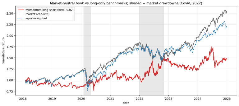
- [§3.4, §4] Section 3.4 states that the one-month return rank is near-random, that covariates add nothing to the return-rank point forecast at any window, and that 'the next-month return of the top decile minus the bottom ... never a positive forward edge' at any ranking window. Section 4 then reports that the market-neutral long-short selected by π_R of Eq. (20) — with λ=0, so the volatility score drops out — has a 'real gross edge' (Sharpe 0.17) and an out-of-sample Sharpe of 0.63. Since §3.4 says the covariates add nothing and the book ranks on a six-month return window, π_R should be nearly equivalent to the trailing-return decile, making the traded long-short exactly the top-minus-bottom spread that §3.4 reports as never positive. This is a load-bearing internal inconsistency: either the §3.4 statistic is computed on a different object than the traded book, or the long-short's edge comes from a
- [§5, Table 11] The statistical support for the headline claim is weak and not adjusted for multiple testing. The clean-window base-book excess-return p-value is 0.09, and the full-record base-book p-value is 0.08; only the diversified clean-window estimate reaches p=0.04. No correction is made for the many variants, periods, and refinements examined in Sections 4–5 and Appendices A–C. Moreover, the abstract's Sharpe comparisons (1.32 versus 1.14, 1.44 versus 1.14) are never tested; the bootstrap addresses only mean excess return. The paper should either provide multiple-testing-adjusted or pre-registered significance statements, report confidence intervals for the Sharpe differences, or temper the abstract's claims of beating the market.
- [§4.1, Table 5] The attribution of the long-only sleeve's contribution is unresolved. Table 5 shows that the long-only book's Sharpe is essentially flat in book size on the validation period and first test, and that the gain on the 2025–2026 window is 'market breadth, not selection alpha.' Because the combined book is fully long-only in rising markets (θ=1), the clean-window Sharpe of 1.44 could owe substantially to holding a broad equal-weight set of names in a strong bull market rather than to the return-chain forecasts. The paper should decompose the combined book's excess return into cap-weight market, equal-weight breadth, and selection/risk-tilt components to show what the three-matrix forecasts actually add.
minor comments (5)
- [Fig. 10] The text says the no-band long-short has a Sharpe of 0.17, while the Figure 10 caption reports 0.13. Please reconcile.
- [§5] The abstract calls both test sets 'non-overlapping out-of-sample,' but §5 concedes that the 2022–2024 period was used repeatedly to refine the book and is 'no longer perfectly clean.' Please qualify the first test in the abstract.
- [§2.1] The distance matrix is N×N with N varying as the S&P 500 constituent list changes; calling the three matrices 'fixed-size' is misleading. Clarify that only the transition-matrix dimensions are fixed.
- [§5] The Yahoo panel of 'the 475 names with a full history since 2018' still induces survivorship for the 2022–2024 cross-source slice and for the beginning of the clean window. The paper acknowledges a mild survivorship tilt for the earlier slice; please quantify the effect on the clean window as well.
- [General] The code repository is currently private. For a paper whose central claim is a strong empirical outperformance, public code and data or a detailed pseudocode appendix are important for verification.
Circularity Check
No circularity: the out-of-sample performance is measured, not derived from fitted inputs; the return-chain tension is a validity concern, not a circular reduction.
full rationale
The paper's derivation chain runs from the three-matrix state (Eqs. 1-5), to covariate-conditioned chains (Eqs. 10-16), to the selection scores pi_R and pi_V (Eqs. 20-21), and then to the portfolio construction of Section 4 and the out-of-sample tests of Sections 4-5. At no point does any equation use the market-beating result or the reported Sharpe as an input. The hyperparameters are chosen on the validation period through 2021 and held fixed out of sample; the chain coefficients are refit walk-forward, so no future observation enters a forecast. The convexity bound sigma_cond >= sigma (Eq. 18) is proved by Jensen's inequality applied to the KL divergence, which is standard mathematics rather than a self-imported uniqueness claim. The paper relies on the author's earlier OMD-Stocks and OMD work for the representation and for diagnostic tools, but the portfolio's outperformance is measured against the capitalization-weighted market on two non-overlapping test sets, including a clean window built from an independent data source with frozen hyperparameters. Those citations therefore do not carry the load of the performance claim. The apparent inconsistency between Section 3.4's finding that the next-month return spread of the top decile minus the bottom is never positive and Section 4's reported positive out-of-sample long-short Sharpe is a substantive internal-consistency and attribution question about where the edge comes from, but it is not a circular step: the reported Sharpe is not constructed to equal pi_R or any other fitted quantity. Correctness risk and circularity are distinct, and this paper's central empirical claim is self-contained against external benchmarks.
Assumptions & free parameters
free parameters (8)
- Book size K =
15
- No-trade tolerance tol =
0.08
- Regime weight lambda =
0 in rising markets, 0.75 in falling
- Blend weight theta =
1 in rising markets, 0.4 in falling
- Diversification tilt gamma =
0.5
- Return ranking window tau_R =
6 months
- Volatility lookback for return-chain predictor =
63 days
- Hub overlay weight =
0.25
assumptions (6)
- standard math KL divergence joint convexity implies sigma_cond >= sigma (Eq. 18).
- standard math The conditional-logit negative log-likelihood is convex and the matrix exponential defines valid transition probabilities (Eqs. 10-15).
- domain assumption The arccos of the Pearson correlation is a geodesic distance on the unit sphere and captures cross-sectional geometry (Eq. 1).
- domain assumption Cross-sectional decile rank-bucketing preserves the tradeable information of each characteristic (Eq. 9).
- domain assumption Monthly ranking dynamics are approximately Markov within each walk-forward refit window.
- domain assumption Transaction costs are 5bp per name traded, with no short-borrow or stress market-impact costs.
Cite this review
Pith. "Pith review of Are Three Matrices All You Need To Beat the Market? Observable Matrix Dynamics for Portfolio Optimization." pith.science (2026). https://pith.science/paper/QRSLOEQI
@misc{pith2026260727461,
  author       = {Pith},
  title        = {Pith review of: Are Three Matrices All You Need To Beat the Market? Observable Matrix Dynamics for Portfolio Optimization},
  year         = {2026},
  howpublished = {\url{https://pith.science/paper/QRSLOEQI}},
  note         = {Machine review of arXiv:2607.27461}
}
abstract
We present a simple framework for dynamic portfolio management that uses nothing but daily prices, trading volumes, and market capitalizations. Its state is three fixed-size matrices built from the price history: the distance matrix of the return correlations and the transition matrices of two Markov chains that rank the S\&P 500 names monthly by trailing return and by trailing volatility. These three matrices rest on the price history alone, the same information Markowitz mean-variance optimization draws on, but they replace its expected-return vector and covariance matrix. Our method requires no matrix inversion, works on outlier-robust cross-sectional ranks, and is dynamic rather than single-period. Empirically the volatility rank is forecastable one step ahead while the return rank stays close to unforecastable. A portfolio built on the forecasts, a market-neutral momentum long-short blended with an opportunistic long-only sleeve, beats the market on two non-overlapping out-of-sample test sets, January 2022 to December 2024 and January 2025 to July 2026, at Sharpes of $1.06$ and $1.32$ against the market's $0.78$ and $1.14$, respectively, net of a five-basis-point trading cost and marked to market daily. It also outperforms the classical minimum-variance and maximum-diversification portfolios. Diversifying the long sleeve by residual distance adds a further edge on both periods, lifting the Sharpe to $1.08$ and $1.44$ and the annualized return from $18\%$ to $20\%$ and from $44\%$ to $56\%$, respectively. A convex information-leader overlay separately insures the market-neutral sleeve, buying convexity and a shallower drawdown at a small cost in return, the Sharpe unchanged.
Figures


Figures from the paper (20 more)




Reference graph
Works this paper leans on
-
[1]
Vaswani, N
A. Vaswani, N. Shazeer, N. Parmar, J. Uszkoreit, L. Jones, A. N. Gomez, L. Kaiser, and I. Polo- sukhin.Attention Is All You Need. Advances in Neural Information Processing Systems30(2017)
2017
-
[2]
Halperin.Observable Matrix Dynamics of Stocks.arXiv:2607.19005 (2026)
I. Halperin.Observable Matrix Dynamics of Stocks.arXiv:2607.19005 (2026)
arXiv 2026
-
[3]
E. F. Fama.Efficient Capital Markets: A Review of Theory and Empirical Work. The Journal of Finance25(2), 383–417 (1970)
1970
-
[4]
M. F. Dixon, I. Halperin, and P. Bilokon.Machine Learning in Finance: From Theory to Practice. Springer, 2020
2020
-
[5]
Markowitz.Portfolio Selection
H. Markowitz.Portfolio Selection. The Journal of Finance7(1), 77–91 (1952)
1952
-
[6]
Clarke, H
R. Clarke, H. de Silva, and S. Thorley.Minimum-Variance Portfolio Composition. The Journal of Portfolio Management37(2), 31–45 (2011)
2011
-
[7]
Choueifaty and Y
Y. Choueifaty and Y. Coignard.Toward Maximum Diversification. The Journal of Portfolio Man- agement35(1), 40–51 (2008)
2008
-
[8]
I. Halperin.Learning as Observable Matrix Dynamics: Diffusive Relaxations versus Phase Transi- tions.arXiv:2606.29679 (2026)
arXiv 2026
Show all 26 references
-
[9]
E. R. Fernholz.Stochastic Portfolio Theory.Springer, New York (2002)
2002
-
[10]
A. D. Banner, R. Fernholz, and I. Karatzas.Atlas Models of Equity Markets. Annals of Applied Probability15(4), 2296–2330 (2005)
2005
-
[11]
Halperin.I-BBS: Inference of Latent Sub-Manifolds in Representation Spaces Using Random Distance Matrices.2026
I. Halperin.I-BBS: Inference of Latent Sub-Manifolds in Representation Spaces Using Random Distance Matrices.2026
2026
-
[12]
Bogomolny, O
E. Bogomolny, O. Bohigas, and C. Schmit. Spectral properties of distance matrices.Journal of Physics A: Mathematical and General36, 3595–3616 (2003). arXiv:nlin/0301044
2003 arXiv
-
[13]
Bogomolny, O
E. Bogomolny, O. Bohigas, and C. Schmit.Distance matrices and isometric embeddings. arXiv:0710.2063 (2007)
-
[14]
Halperin.Frustrated Dynamics of Distance Matrices.arXiv:2605.05376 (2026)
I. Halperin.Frustrated Dynamics of Distance Matrices.arXiv:2605.05376 (2026)
2026 arXiv
-
[15]
Lando and T
D. Lando and T. M. Skødeberg.Analyzing Rating Transitions and Rating Drift with Continuous Observations. Journal of Banking and Finance26(2–3), 423–444 (2002)
2002
-
[16]
Kavvathas.Estimating Credit Rating Transition Probabilities for Corporate Bonds.Working paper, University of Chicago, 2001
D. Kavvathas.Estimating Credit Rating Transition Probabilities for Corporate Bonds.Working paper, University of Chicago, 2001
2001
-
[17]
Schreiber.Measuring Information Transfer
T. Schreiber.Measuring Information Transfer. Physical Review Letters85, 461–464 (2000)
2000
-
[18]
R. Quax, D. Kandhai, and P. M. A. Sloot.Information Dissipation as an Early-Warning Signal for the Lehman Brothers Collapse in Financial Time Series. Scientific Reports3, 1898 (2013)
2013
-
[19]
Akiba, S
T. Akiba, S. Sano, T. Yanase, T. Ohta, and M. Koyama.Optuna: A Next-generation Hyperparam- eter Optimization Framework. Proc. 25th ACM SIGKDD International Conference on Knowledge Discovery and Data Mining, 2623–2631 (2019)
2019
-
[20]
Daniel and T
K. Daniel and T. J. Moskowitz.Momentum Crashes.Journal of Financial Economics122(2), 221– 49 247 (2016)
2016
-
[21]
Barroso and P
P. Barroso and P. Santa-Clara.Momentum Has Its Moments.Journal of Financial Economics 116(1), 111–120 (2015)
2015
-
[22]
Baltas.The Impact of Crowding in Alternative Risk Premia Investing
N. Baltas.The Impact of Crowding in Alternative Risk Premia Investing. Financial Analysts Journal 75(3), 89–104 (2019)
2019
-
[23]
Zlotnikov, J
V. Zlotnikov, J. Liu, I. Halperin, F. He and L. L. Huang.Model-Free Market Risk Hedging Using Crowding Networks. The Journal of Portfolio Management50(9), 132–141 (2024)
2024
-
[24]
Jegadeesh and S
N. Jegadeesh and S. Titman.Returns to Buying Winners and Selling Losers: Implications for Stock Market Efficiency. The Journal of Finance48(1), 65–91 (1993)
1993
-
[25]
T. I. Jensen, B. T. Kelly, and L. H. Pedersen.Is There a Replication Crisis in Finance? Journal of Finance78(5), 2465–2518 (2023)
2023
-
[26]
S. V. George, S. Kachhara, and G. Ambika.Early Warning Signals for Critical Transitions in Complex Systems. Physica Scripta98, 072002 (2023). arXiv:2107.01210. 50
2023 arXiv
Reviewed August 1, 2026 · model on record in the stance chip above.
Discussion (0). Continue with ORCID to comment.