REVIEW 3 major objections 4 minor 290 references
Structured coherence: A modern perspective on optical coherence as a resource
T0 review · 3 major / 4 minor · reviewed 2026-08-07 · deepseek-v4-flash
Pith's one-line read The paper argues that partially coherent light, captured by a coherence matrix, can outperform coherent light in optical information processing.
desk verdict A clear, useful tutorial whose 'coherence advantage' is a real but narrowly-scoped effect, not the general resource the title implies. read the letter →
The pith
A machine-rendered reading of the paper's core claim, the machinery that carries it, and where it could break.
The reading
What carries the argument
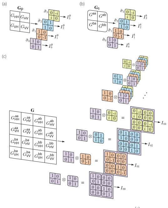
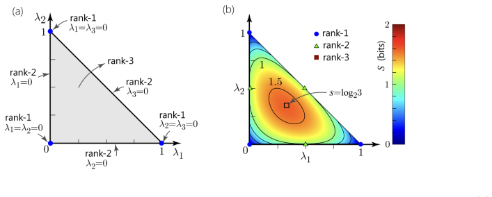
The load-bearing object is the $N\times N$ coherence matrix $G = \langle E_j E_k^*\rangle$, a Hermitian, positive-semidefinite, unity-trace matrix obtained by averaging outer products of the random modal amplitudes over the ensemble. Everything else hangs on how $G$ transforms: unitary operations $G \rightarrow U G U^\dagger$ (which are reversible and preserve entropy and degree of coherence), non-unitary filtering and decohering operators (which tune them), the partial trace that produces reduced spatial and polarization coherence matrices from a $4\times 4$ $G$, and the scalar diagnostics — degree of coherence $D = \lambda_1 - \lambda_2$, entropy $S = -\operatorname{Tr}(G \log_2 G)$, coherence rank (the number of nonzero eigenvalues), and optical cross-purity. These objects turn 'how much the field fluctuates' into quantitative, manipulable resources.
What would settle it
Take a rapidly varying, strongly scattering polarization channel. Encode bits as $0 \rightarrow |H\rangle$ (degree of polarization 1) and $1 \rightarrow$ a maximally unpolarized field (degree of polarization 0), and decode by thresholding the degree of polarization at 0.5. If the measured cross-talk matrix is not diagonal, meaning the bit-error rate is no better than encoding 0 and 1 in orthogonal polarized states, then the claimed coherence advantage for this channel is falsified.
Extended reading notes
Core claim
On the paper's own terms, the claim it is trying to secure is that partial coherence is not noise to be eliminated but a structured resource: in a fixed, orthonormal, closed modal basis, the coherence matrix $G = \langle E_j E_k^*\rangle$ completely characterizes the fluctuating field, and its properties — degree of coherence, von Neumann entropy, coherence rank (the number of nonzero eigenvalues), and cross-purity between degrees of freedom — determine what can and cannot be done with the field. Because a coherent $N$-mode field needs only $2N-2$ real parameters while a partially coherent one needs $N^2-1$, partially coherent fields carry more information per field; because the degree of coherence or rank can be made immune to scattering that destroys polarization states, encoding in these quantities enables communication through channels where coherent encoding fails. The tutorial systematizes the unitary, filtering, and decohering operations that manipulate the coherence matrix, showing how entropy can be swapped between degrees of freedom, concentrated into modes, or spread across them.
Load-bearing premise
The load-bearing premise is that the field is fully captured by a fixed, finite, closed set of orthonormal modes, so that randomness enters only through the complex modal amplitudes and no modes outside the basis ever contribute.
Editorial extensions
If this is right
- A partially coherent field in $N$ modes occupies $N^2-1$ real parameters, so partial coherence enlarges the information-carrying capacity of an optical field relative to coherent encoding.
- Encoding bits in the degree of coherence (polarized versus unpolarized) survives a channel that randomly rotates polarization, where encoding bits in orthogonal polarization states fails.
- Coherence rank becomes a communication resource: the number of nonzero eigenvalues of the coherence matrix can carry information through strongly scattering channels.
- Entropy can be moved between degrees of freedom, concentrated into a selected mode, or spread out, which means partial coherence can be deliberately redistributed rather than merely suppressed.
- The $4\times 4$ coherence matrix of two binary degrees of freedom is isomorphic to a two-qubit density matrix, so partial trace, entropy inequalities, and non-separability (classical entanglement) transfer directly to classical optical fields.
Reading between the lines
- Editorial inference: the resource view suggests a quantitative definition of 'coherence advantage' as the ratio of achievable information rates under a fixed channel, with the testable prediction that the advantage grows with modal dimension $N$.
- Editorial inference: optical cross-purity and entropy swapping, developed for two binary degrees of freedom, are natural candidates for on-chip demonstrations with programmable interferometers, which would test the claim on integrated platforms without free-space alignment.
- Editorial inference: if the coherence advantage holds, the practical bottleneck moves to mode-selective measurement; the paper's modal-projector and modal-analyzer toolbox is precisely that missing hardware, and the next step is extending those devices from coherent to partially coherent inputs.
Editorial analysis
A structured set of objections, weighed in public.
Referee Report
Summary. This tutorial proposes 'structured coherence' as the regime in which an optical field is carried by a fixed, finite, deterministic modal basis and all randomness resides in the complex modal coefficients. It develops the associated coherence-matrix formalism: 2x2 matrices for one binary degree of freedom, Stokes parameters and Pauli decompositions, unitary and non-unitary transformations, degree of coherence and entropy, and explicit measurement strategies. It then extends the formalism to two binary degrees of freedom via 4x4 coherence matrices, partial trace, coherence rank, entropy swapping, optical cross-purity, tomographic reconstruction, and a communications protocol across a strongly scattering channel. The paper's motivating claim is a 'coherence advantage': settings in which partially coherent light, described by coherence matrices, can outperform coherent light in optical information processing.
Significance. If the coherence-advantage claim is sustainable, this matrix-based resource perspective could provide a valuable unifying framework for partial coherence in on-chip photonics, multimode fibers, and information processing. The tutorial's linear-algebra core is standard, internally consistent, and clearly presented; it gives explicit reconstruction procedures (Section IV.F), concrete measurement strategies (Section II.C and Section III.D), and an unusually candid statement of channel assumptions (Section III.I). The mathematical formulation itself is a useful pedagogical contribution. However, the central 'coherence advantage' is not derived in the tutorial; it is supported by idealized channel models and by references to the authors' own experimental work. The paper would be strengthened by a clear separation between the sound tutorial mathematics and the status of the advantage claim.
major comments (3)
- [II.A and III.I] The central 'coherence advantage' claim is load-bearing, yet every supporting scenario assumes a closed finite modal basis and, for the communications protocol, a unitary Channel-1. Section II.A defines a closed basis as one in which 'no new modes outside the basis can contribute to the field' and immediately concedes that an infinite basis is typically required and truncation is a practical expedient. Section III.I's assumptions (single-DoF channel, unitarity, no memory) are exactly what makes the maximally incoherent state invariant and what makes the degree of coherence and coherence rank unitarily invariant. If the channel couples the polarization DoF to an unused spatial mode, the reduced 2x2 coherence matrix no longer evolves unitarily: its degree of coherence and rank can change, and the decision threshold in Fig. 33 fails. The tutorial provides no error bound, leakage model, or demonstration of robustness to small violations of the closure assumption. Please add a quantitative robustness discussion or explicitly restrict the coherence-advantage claim to the idealized closed-basis unitary-channel setting.
- [I.D] The parameter-counting argument compares the 2N-2 real parameters needed for a coherent N-mode field with the N^2-1 real parameters needed for a partially coherent field and suggests 'richer information-carrying capacity.' Counting parameters of a state space is not by itself a communication-theoretic advantage: a larger state space can also imply greater noise sensitivity and more demanding measurements, and no coding theorem is given. The text itself concedes that no experiment has exploited this parameter-counting opportunity to date. I recommend reframing this point as an open question rather than as evidence for the coherence advantage.
- [IV.K and IV.M] Entropy swapping and coherence-rank communications are introduced as key applications and as part of the coherence-advantage narrative, but their derivations are not present in the tutorial; the text defers to earlier work (e.g., Refs. [134, 138-142]). The reader therefore cannot inspect the conditions under which coherence rank, entropy, or the reduced coherence matrices are preserved. At a minimum, the tutorial should state the relevant theorems and their explicit assumptions, and it should identify which steps rely on the closed-basis and unitary-channel idealizations. Without that, the claimed advantage remains an assertion about the authors' own protocols rather than a demonstrated result of the presented formalism.
minor comments (4)
- [IV.F Eq. (122)] The (3,3) entry of the reconstructed matrix reads "s00 + s01 - s01 - s11", which is inconsistent with the Kronecker-Pauli expansion; it should be "s00 + s01 - s10 - s11".
- [III.I] The acronym for the cross-talk matrix is given as "CTM" in the text and figures, but later appears as "CMT" in the sentence reporting the flat matrix; please unify the usage.
- [II.D] The claim that the described modal projectors and analyzers are 'equally applicable to partially coherent light' is asserted without a supporting argument or reference; a short explanation of why the linearity of the modal projectors suffices for coherence matrices would be useful.
- [III.C.6] The statement that any two 2x2 coherence matrices with the same entropy can be interconverted by a unitary is correct for the qubit case, but the converse statement for higher-dimensional coherence matrices is only hinted at; a one-sentence caveat would avoid overgeneralization.
Circularity Check
No significant circularity: the tutorial's derivations are self-contained linear algebra; self-citations are pointers, not load-bearing premises.
full rationale
The paper's central derivation chain starts from explicit definitions: the coherence matrix G = integral of P(xi)|E(xi)><E(xi)| over the ensemble, unitary evolution G -> U G U†, degree of coherence D = lambda1 - lambda2, and coherence rank as the number of nonzero eigenvalues. The claimed 'coherence advantage' examples, including the parameter-counting argument, the Channel-1 communications protocol, and coherence-rank transmission, are mathematical consequences of these definitions together with the explicitly stated channel assumptions (e.g., 2x2 unitary scattering). No parameter is fitted to data and then presented as a prediction; the experimental confirmation in Fig. 34 implements the same unitary-channel model and verifies the derived invariance of the degree of polarization. Self-citations such as [134] and [138-142] point to the authors' prior demonstrations, but the necessary mathematics (unitary invariants, partial trace, Stokes reconstruction) is re-derived in the text, so the central claim does not reduce to those citations. The closed-modal-basis and unitarity assumptions are stated idealizations; their failure in realistic systems is a scope and robustness concern, not a circularity in the derivation. No step was found in which an output quantity is identical by construction to an input quantity or in which a fitted parameter is renamed a prediction.
Assumptions & free parameters
assumptions (5)
- domain assumption The optical field is represented in a finite, closed, orthonormal modal basis; no modes outside the basis contribute.
- domain assumption All statistical information about the partially coherent field is captured by ensemble-averaged second-order correlations of modal coefficients.
- domain assumption The field is paraxial, so polarization is a two-dimensional transverse degree of freedom.
- standard math Hermitian matrices admit spectral decomposition, Pauli matrices span 2x2 Hermitian matrices, and the partial trace is trace-preserving.
- domain assumption Relevant optical transformations are unitary, filtering, or decohering maps on the coherence matrix.
Cite this review
Pith. "Pith review of Structured coherence: A modern perspective on optical coherence as a resource." pith.science (2026). https://pith.science/paper/VGL42G3O
@misc{pith2026260806356,
  author       = {Pith},
  title        = {Pith review of: Structured coherence: A modern perspective on optical coherence as a resource},
  year         = {2026},
  howpublished = {\url{https://pith.science/paper/VGL42G3O}},
  note         = {Machine review of arXiv:2608.06356}
}
read the original abstract
Optical coherence is a well-established branch of physical optics in which the statistical properties of fluctuating optical fields are described in terms of correlation functions over continuous spatial and temporal degrees of freedom (DoFs). Nevertheless, in any practical setting, only discrete DoFs are ever accessible. In these scenarios, the modes are fixed, stable, and deterministic, and partial coherence arises from random relative complex amplitudes, a configuration we refer to as 'structured coherence'. Advances in structured coherence have recently unveiled new conceptual ground in optical communications and information processing in which partial coherence may be preferable to full coherence, which we call a 'coherence advantage'. We formulate structured coherence in terms of coherence matrices to investigate these recent theoretical and experimental breakthroughs. We first review optical fields characterized by a binary DoF via 2x2 Hermitian coherence matrices and introduce key concepts that take on new significance for larger-dimensional modal sets. Next, we examine the structured coherence of two binary DoFs, which can be described by 4x4 coherence matrices. We introduce the concept of coherence rank, entropy swapping, and optical cross-purity. In the perspective outlined here, coherence is viewed as a 'resource', which can be exchanged between DoFs, concentrated into a DoF or into particular modes, or spread over the DoFs. We then examine larger-dimensional modal sets, which allow for more versatile applications in optical information processing. The formulation presented here lends itself particularly to the manipulation of partial optical coherence in integrated photonic platforms, thereby opening myriad avenues for novel fundamental investigations of structured coherence and exploiting the coherence advantage in optical communications and information processing.
Figures


Figures from the paper (61 more)






Reference graph
Works this paper leans on
-
[1]
Mandel in 1961 using the conventional description of optical coherence in terms of continuous functions in space and time
Basic definition Spectral cross-purity is a phenomenon first described by L. Mandel in 1961 using the conventional description of optical coherence in terms of continuous functions in space and time. Consider superposing the spectra from points |a⟩ and |b⟩, Sa(ω) and Sb(ω), respectively, in a scalar, partially coherent field. If the spectra Sa(ω) and Sb(ω...
1961
-
[2]
Symmetry: the normalized spectra at |a⟩ and |b⟩ are identical
-
[3]
Separability: The coherence function at these two points is independent of the spatial coordinate; i.e., the coherence function is separable with respect to the spatial and spectral DoFs at these two points. The fundamental concept of cross-spectral purity has been recently generalized in two aspects: (1) it can be applied to any pair of DoFs; and (2) it ...
-
[4]
Polarization cross-purity We apply generalized optical cross-purity to a scenario comprising the spatial and polarization DoFs. We thus consider the following question: in a partially coherent vector field described by a 4 × 4 coherence matrix G, in which the polarizations at |a⟩ and |b⟩ are identical, would superposing the fields from |a⟩ and |b⟩ yield t...
-
[5]
55(a)], we instead implement a unitary operator ˆUs that impacts the spatial DoF alone and is independent of polarization DoF [Fig
Conditions for polarization cross-purity Rather than superposing the fields from |a⟩ and |b⟩ in the double-slit experiment [Fig. 55(a)], we instead implement a unitary operator ˆUs that impacts the spatial DoF alone and is independent of polarization DoF [Fig. 55(b)]. We start with the block-matrix form for the coherence matrix G = |α|2Ga Gab Gba |β|2Ga ,...
-
[6]
Optical cross-purity and the coherence rank Evaluating cross-purity requires first symmetrizing the field so that Ga = Gb. Once the field is symmetrized, is it guaranteed to be separable? Does symmetry ( Ga = Gb) imply separability (and thus polarization cross-purity)? We have recently shown that the coherence rank [134, 141, 142] is crucial in this regar...
-
[7]
Consequently, even if G3 = ˆU GD 3 ˆU † is symmetrized ( Ga = Gb), G3 remains non-separable
Rank-3 fields are intrinsically non-separable [142]; no unitary transformation can undo this non-separability. Consequently, even if G3 = ˆU GD 3 ˆU † is symmetrized ( Ga = Gb), G3 remains non-separable. That is, all rank-3 fields are polarization cross-impure ; in this case, symmetry does not imply separability. 73 We consider an example to clarify the d...
-
[8]
The channel impacts both the polarization and spatial DoFs but not any further DoFs
Show all 290 references
-
[9]
The channel can be represented for any bit during data transmission by a 4 × 4 unitary ˆU that encompasses both the polarization and spatial DoFs
-
[10]
Rapidly varying channel: ˆU changes from bit to bit
-
[11]
Strong scattering:family of 4 × 4 unitaries over both polarization and spatial DoFs
-
[12]
No-memory channel: ˆU at any two moments in time are uncorrelated
-
[13]
This channel scatters polarization strongly, scatters the spatial modes strongly, and moreover couples the polarization and spatial DoFs
An overall loss factor can be included, which is assumed to be independent of polarization and spatial modes. This channel scatters polarization strongly, scatters the spatial modes strongly, and moreover couples the polarization and spatial DoFs. These features vary rapidly f...
-
[14]
The bit pairs 00, 01, 10, and 11 are encoded in coherence matrices G00, G01, G10, and G11, respectively
-
[15]
The physical field is transmitted across the communications channel
-
[16]
At the channel output, G is tomographically reconstructed (by measuring the modal Stokes parameters) and its eigenvalues are estimated
-
[17]
The rank of the coherence matrix is estimated
-
[18]
Bit pairs can then be decoded from the estimated rank: rank-1 → 00, rank-2 → 01, rank-3 → 10, and rank −4 → 11. The difficulty is that imperfections in the synthesis and detection stages, in addition to noise and scattering in the channel, may displace the values of the eigenva...
-
[19]
Establishing scattering-immune communications over a strongly scattering channel
-
[20]
Solving the problem of frame-sharing: the sender and receiver do not need to have the same shared reference system for polarization or spatial modes (e.g., they may not agree on what constitutes |H⟩ and |V⟩
-
[21]
The communication scheme is impervious to any phases introduced between the spatial or polarization modes
-
[22]
Potential limitations of coherence-rank communications are:
Overall losses do not affect the communications scheme. Potential limitations of coherence-rank communications are:
-
[23]
Modal-dependent losses can introduce errors if they are severe enough to change the coherence rank
-
[24]
It fails if the rate of change in the channel is faster than the data rate
-
[25]
The detection process required reconstruction of the coherence matrix G rather than detecting the power directly. The last limitation is currently being alleviated by gradually transitioning to photonic integrated circuits to reconstruct the coherence matrix rather than relyin...
-
[26]
This mathematical analogy can be extended to the two binary-DoF scenario, which is analogous to a two-qubit quantum system
Similarities We explored in Section III J the mathematical analogy between a classical optical field characterized by a binary DoF and a qubit (a two-level quantum-mechanical system). This mathematical analogy can be extended to the two binary-DoF scenario, which is analogous ...
-
[27]
(a) Quantum entanglement is a valuable resource in quantum information processing
Distinctions Whereas there are many formal similarities between the mathematical structures of quantum and classical entan- glement that have been investigated over the past few decades, there nevertheless exist several critical distinctions. (a) Quantum entanglement is a valu...
-
[28]
A coherent field is associated with an N × 1 field vector |E⟩: |E⟩ = 0 BBBBBB@ E1 E2
Coherence matrix for N -mode fields Consider an optical DoF described by a modal basis comprising N > 2 orthonormal modes, {|j⟩}N j=1, so that ⟨j|k⟩ =δjk . A coherent field is associated with an N × 1 field vector |E⟩: |E⟩ = 0 BBBBBB@ E1 E2 ... ... EN 1 CCCCCCA =E1 0 BBBBBB@ 1...
-
[29]
the diagonal elements are real Gjj =G∗ jj
-
[30]
the off-diagonal elements form conjugate pairs Gjk =G∗ kj
-
[31]
the eigenvalues {λ1,λ 2, · · ·,λ N } of G are real
-
[32]
the eigenvectors of G are orthogonal when their associated eigenvalues are different
-
[33]
the coherence matrix can be diagonalized via an N ×N unitary: GD = ˆU G ˆU † = diag{λ1,λ 2, · · ·,λ N }; and
-
[34]
We normalize the coherence matrix to unity trace, Tr{G} =PN j=1Gjj =PN j=1λj = 1
the coherence matrix is positive semi-definite, so that λj ≥ 0 and Gjj ≥ 0. We normalize the coherence matrix to unity trace, Tr{G} =PN j=1Gjj =PN j=1λj = 1. The diagonal elements of G correspond to the fractions of power associated with each mode. The detectors in Fig. 60(a) ...
-
[35]
The N eigenvalues are unitary invariants, while the remaining N (N − 1) ‘angular’ parameters vary with unitaries
Coherent, partially coherent, and incoherent fields The number of real parameters needed to uniquely identify a Hermitian unity-trace N ×N coherence matrix is N 2 − 1. The N eigenvalues are unitary invariants, while the remaining N (N − 1) ‘angular’ parameters vary with unitar...
-
[36]
(149) Such a coherence matrix can be diagonalized by a 3 × 3 unitary ˆU , G(D) = ˆU G3 ˆU †
Example: A three-mode field For concreteness, we consider explicitly the case of a three-mode field ( N = 3) spanned by a modal basis {|1⟩, |2⟩, |3⟩} in which the coherence matrix is expressed as: G = 0 @ G11 G12 G13 G21 G22 G23 G31 G32 G33 1 A. (149) Such a coherence matrix c...
-
[37]
Nevertheless, one scheme that has had significant impact in quantum communications using photons is so-called ‘time-bins’, as depicted in Fig
Temporal modal bases We have focused here on the spatial and polarization DoFs, but the matrix formulation for structured coherence is equally applicable to any DoF, including the temporal and spectral DoFs, although it is much less common there. Nevertheless, one scheme that ...
-
[38]
Two examples of discrete modal bases for the spectral DoF are given in Fig
Spectral modal bases Similarly to the case of temporal modes, only limited interest has been directed to spectral modal bases. Two examples of discrete modal bases for the spectral DoF are given in Fig. 62(c,d), both of which can be classified as non-overlapping modes. In Fig....
-
[39]
Tuning the coherence rank by setting the requisite amplitudes to zero
-
[40]
Adjusting the entropy of the field by varying the values of the non-zero eigenvalues
-
[41]
Sculpting the coherence matrix by implementing the requisite N ×N unitary ˆU , comprising a sequence of 2 × 2 unitaries operating on pairs of modes. Once the target coherence matrix Gin is synthesized on chip, the field is launched into a physical optical channel, where all th...
-
[42]
B. E. A. Saleh and M. C. Teich, Fundamentals of Photonics (Wiley, 2007)
2007
-
[43]
Mashaal, A
H. Mashaal, A. Goldstein, D. Feuermann, and J. M. Gordon, Opt. Lett. 37, 3516 (2012)
2012
-
[44]
Divitt and L
S. Divitt and L. Novotny, Optica 2, 95 (2015)
2015
-
[45]
Dellieu, G
L. Dellieu, G. Cael, M. Louette, A. Herman, O. Deparis, and M. Sarrazin, Mater. Today Proc. 4, 4952 (2017)
2017
-
[46]
Vow Ricketti, E
B. Vow Ricketti, E. M. Gauger, and A. Fedrizzi, Sci. Rep. 12, 5438 (2022)
2022
-
[47]
A. A. Michelson, Phil. Mag. 30, 1 (1890)
-
[48]
A. A. Michelson and F. G. Pease, Astrophys. J. 53, 249 (1921)
1921
-
[49]
Zagury and P
F. Zagury and P. Pellat-Finet, Opt. Commun. 285, 4001 (2012)
2012
-
[50]
Hanbury-Brown and R
R. Hanbury-Brown and R. Q. Twiss, Nature 178, 1046 (1956)
1956
-
[51]
Hanbury-Brown, The Intensity Interferometer: Its Application to Astronomy (Taylor & Francis, London, 1974)
R. Hanbury-Brown, The Intensity Interferometer: Its Application to Astronomy (Taylor & Francis, London, 1974)
1974
-
[52]
P. K. Tan, G. H. Yeo, H. S. Poh, A. H. Chan, and C. Kurtsiefer, Astrophys. J. Lett. 789, L10 (2014)
2014
-
[53]
C. W. Tang and S. A. Van Slyke, Appl. Phys. Lett. 51, 913 (1987)
1987
-
[54]
Y. A. Ono, Electroluminescent Devices (World Scientific, Singapore, 1995)
1995
-
[55]
D. R. Vij, ed., Luminescence of Solids (Springer, 1998). 84
1998
-
[56]
Wilson and J
T. Wilson and J. W. Hastings, Annu. Rev. Cell Dev. Biol. 14, 197 (1998)
1998
-
[57]
B. J. M. Brenny, T. Coenen, and A. Polman, J. Appl. Phys. 115, 244307 (2014)
2014
-
[58]
J. R. Lakowicz, Principles of Fluorescence Spectroscopy (Springer, 2006)
2006
-
[59]
Diaspro, ed., Optical Fluorescence Microscopy: From the Spectral to the Nano Dimension (Springer, Berlin, 2011)
A. Diaspro, ed., Optical Fluorescence Microscopy: From the Spectral to the Nano Dimension (Springer, Berlin, 2011)
2011
-
[60]
H. O. Anger, Rev. Sci. Instrum. 29, 27 (1958)
1958
-
[61]
J. L. Codona and R. G. Frehlich, Radio Sci. 22, 469 (1987)
1987
-
[62]
Wesemann, J
W. Wesemann, J. Opt. Soc. Am. A 4, 1439 (1987)
1987
-
[63]
Sahin, Appl
S. Sahin, Appl. Opt. 64, 957 (2025)
2025
-
[64]
H. Lu, O. Alkhazragi, Y. Wang, N. Almaymoni, W. Yan, W. H. Gunawan, H. Lin, T.-Y. Park, T. K. Ng, and B. S. Ooi, npj Nanophoton. 1, 9 (2024)
2024
-
[65]
M. J. Beran, J. Opt. Soc. Am. 60, 518 (1970)
1970
-
[66]
R. L. Fante, J. Opt. Soc. Am. 64, 592 (1974)
1974
-
[67]
R. L. Fante, Proc. IEEE 63, 1669 (1975)
1975
-
[68]
Gbur and E
G. Gbur and E. Wolf, J. Opt. Soc. Am. A 19, 1592 (2002)
2002
-
[69]
S. A. Ponomarenko and E. Wolf, Opt. Lett. 27, 1770 (2002)
2002
-
[70]
Dogariu and S
A. Dogariu and S. Amarande, Opt. Lett. 28, 10 (2003)
2003
-
[71]
Shirai, A
T. Shirai, A. Dogariu, and E. Wolf, J. Opt. Soc. Am. A 20, 1094 (2003)
2003
-
[72]
Korotkova, L
O. Korotkova, L. C. Andrews, and R. L. Phillips, Opt. Eng. 43, 330 (2004)
2004
-
[73]
G. P. Berman and A. A. Chumak, Phys. Rev. A 71, 013805 (2006)
2006
-
[74]
G. P. Berman, A. A. Chumak, and V. N. Gorshkov, Phys. Rev. E 76, 056606 (2007)
2007
-
[75]
F. Wang, X. Liu, and Y. Cai, Prog. Electromag. Res. 150, 123 (2015)
2015
-
[76]
M. A. Cox, N. Mphuthi, I. Nape, N. Mashaba, L. Cheng, and A. Forbes, IEEE J. Sel. Top. Quant. Electron. 27, 7500521 (2020)
2020
-
[77]
R. R. Alfano, W. B. Wang, L. Wang, and S. K. Gayen, in Photonics: Biomedical Photonics, Spectroscopy, and Microscopy , edited by D. L. Andrews (John Wiley & Sons, 2015) pp. 367–412
2015
-
[78]
D. D. Nolte, Rep. Prog. Phys. 87, 036601 (2024)
2024
-
[79]
S. E. Orchard, J. Oil Colour Chem. Assoc. 54, 44 (1968)
1968
-
[80]
W. E. Vargas, P. Greenwood, J. E. Otterstedt, and G. A. Niklasson, Solar Energy 68, 553 (2000)
2000
-
[81]
Auger and B
J.-C. Auger and B. Stout, J. Coatings Technol. Res 9, 287 (2012)
2012
-
[82]
Fujii and T
H. Fujii and T. Asakura, Nouvelle Revue d’Optique 6, 5 (1975)
1975
-
[83]
J. W. Goodman, Speckle Phenomena in Optics (Roberts and Company Publishers, Colorado, 2007)
2007
-
[84]
Y. Peng, S. Choi, J. Kim, and G. Wetzstein, Sci. Adv. 7, eabg5040 (2021)
2021
-
[85]
Evered, K
C. Evered, K. Li, Y. Fan, B. Zhang, and A. Roula, Opt. Laser Technol. 183, 112407 (2025)
2025
-
[86]
M. Z. Islam, S. Ekin, and J. F. O’Hara, arXiv:2304.09922 (2023)
2023 arXiv
-
[87]
Deng and D
Y. Deng and D. Chu, Sci. Rep. 7, 5893 (2017)
2017
-
[88]
Akcay, P
C. Akcay, P. Parrein, and J. P. Rolland, Appl. Opt. 41, 5256 (2002)
2002
-
[89]
Young, Phil
T. Young, Phil. Trans. R. Soc. 94, 1 (1804)
-
[90]
Kipnis, History of the Principle of Interference of Light (Springer, Basel, 1991)
N. Kipnis, History of the Principle of Interference of Light (Springer, Basel, 1991)
1991
-
[91]
A. I. Sabra, Theories of Light from Descartes to Newton (Cambridge Univ. Press, 1981)
1981
-
[92]
A. A. Michelson, Phil. Mag. 31, 256 (1891)
-
[93]
A. A. Michelson, Phil. Mag. 31, 338 (1891)
-
[94]
A. A. Michelson, Phil. Mag. 32, 280 (1892)
-
[95]
Zernicke, Physica 5, 785 (1938)
F. Zernicke, Physica 5, 785 (1938)
1938
-
[96]
Laue, Ann
M. Laue, Ann. der Physik 23, 1 (1907)
1907
-
[97]
Berek, Z
M. Berek, Z. Physik 37, 387 (1926)
1926
-
[98]
Wiener, Acta Math
N. Wiener, Acta Math. 55, 117 (1930)
1930
-
[99]
P. H. Van Cittert, Physica 6, 1129 (1939)
1939
-
[100]
H. H. Hopkins, Proc. Roy. Soc. A 208, 263 (1951)
1951
-
[101]
Wolf, Nature 172, 535 (1953)
E. Wolf, Nature 172, 535 (1953)
1953
-
[102]
Wolf, Nuovo Cimento 12, 884 (1954)
E. Wolf, Nuovo Cimento 12, 884 (1954)
1954
-
[103]
Wolf, Proc
E. Wolf, Proc. Roy. Soc. A 225, 96 (1954)
1954
-
[104]
Wolf, Proc
E. Wolf, Proc. Roy. Soc. A 230, 246 (1955)
1955
-
[105]
Wolf, Phil
E. Wolf, Phil. Mag. 2, 351 (1957)
1957
-
[106]
Wolf, Il Nuovo Cimento 13, 1165 (1959)
E. Wolf, Il Nuovo Cimento 13, 1165 (1959)
1959
-
[107]
Mandel and E
L. Mandel and E. Wolf, J. Opt. Soc. Am. 51, 815 (1961)
1961
-
[108]
Mandel and E
L. Mandel and E. Wolf, Rev. Mod. Phys. 37, 231 (1965)
1965
-
[109]
A. F. Forrester, Am. J. Phys. 41, 192 (1956)
1956
-
[110]
Gamo, Oyo Buturi 25, 431 (1956)
H. Gamo, Oyo Buturi 25, 431 (1956)
1956
-
[111]
H. H. Hopkins, J. Opt. Soc. Am. 47, 508 (1957)
1957
-
[112]
G. B. Parrent Jr., J. Opt. Soc. Am. 49, 787 (1959)
1959
-
[113]
G. B. Parrent Jr., Opt. Acta 6, 285 (1959)
1959
-
[114]
E. L. O’Neill and L. Bradley, Phys. Today 14, 28 (1961)
1961
-
[115]
R. N. Bracewell, Proc. IRE 50, 214 (1962)
1962
-
[116]
Martienssen and E
W. Martienssen and E. Spiller, Am. J. Phys. 32, 919 (1964). 85
1964
-
[117]
C. W. McCutchen, J. Opt. Soc. Am. 56, 727 (1966)
1966
-
[118]
Wolf and D
E. Wolf and D. F. V. James, Rep. Prog. Phys. 59, 771 (1996)
1996
-
[119]
A. J. Devaney, A. T. Friberg, A. T. Kumar, and E. Wolf, Opt. Lett. 22, 1672 (1997)
1997
-
[120]
Dorrer, J
C. Dorrer, J. Opt. Soc. Am. 21, 1417 (2004)
2004
-
[121]
Wolf, Introduction to the Theory of Coherence and Polarization of Light (Cambridge Univ
E. Wolf, Introduction to the Theory of Coherence and Polarization of Light (Cambridge Univ. Press, Cambridge, 2007)
2007
-
[122]
A. T. Friberg and T. Setälä, J. Opt. Soc. Am. A 33, 2431 (2016)
2016
-
[123]
Korotkova and G
O. Korotkova and G. Gbur, Prog. Opt. 62, 43 (2020)
2020
-
[124]
Y. Chen, A. Norrman, S. A. Ponomarenko, and A. T. Friberg, Prog. Opt. 62, 105 (2020)
2020
-
[125]
J. Yu, X. Zhu, F. Wang, Y. Chen, and Y. Cai, Prog. Quant. Electron. 91-92, 100486 (2023)
2023
-
[126]
Wolf, Nuovo Cimento 13, 1165 (1959)
E. Wolf, Nuovo Cimento 13, 1165 (1959)
1959
-
[127]
Wolf, Proc
E. Wolf, Proc. Phys. Soc. 76, 424 (1960)
1960
-
[128]
G. B. Parrent Jr. and P. Roman, Nuovo Cimento 15, 370 (1960)
1960
-
[129]
Shurcliff, Polarized Light: Production and Use (Harvard Univ
W. Shurcliff, Polarized Light: Production and Use (Harvard Univ. Press, 1966)
1966
-
[130]
N. M. Azzam and R. M. A. Bashara, Ellipsometry and Polarized Light (North-Holland, 1977)
1977
-
[131]
Brosseau, Fundamentals of Polarized Light (Wiley, New York, 1998)
C. Brosseau, Fundamentals of Polarized Light (Wiley, New York, 1998)
1998
-
[132]
Gamo, Prog
H. Gamo, Prog. Opt. 3, 187 (1964)
1964
-
[133]
E. L. O’Neill and T. Asakura, J. Phys. Soc. Jpn. 16, 301 (1961)
1961
-
[134]
G. Li, N. Bai, N. Zhao, and C. Xia, Adv. Opt. Photon. 6, 413 (2014)
2014
-
[135]
Bogaerts, D
W. Bogaerts, D. Pérez, J. Capmany, D. A. B. Miller, J. Poon, D. Englund, F. Morichetti, and A. Melloni, Nature 586, 207–216 (2020)
2020
-
[136]
A. E. Willner, H. Huang, Y. Yan, Y. Ren, N. Ahmed, G. Xie, C. Bao, L. Li, Y. Cao, Z. Zhao, J. Wang, M. P. J. Lavery, M. Tur, S. Ramachandran, A. F. Molisch, N. Ashrafi, and S. Ashrafi, Adv. Opt. Photon. 7, 66 (2015)
2015
-
[137]
U. Levy, S. Derevyanko, and Y. Silberberg, Prog. Opt. 61, 237 (2016)
2016
-
[138]
A. E. Siegman, Lasers (University Science Books, 1986)
1986
-
[139]
Y. Zhou, J. Zhao, Z. Shi, S. M. H. Rafsanjani, M. Mirhosseini, Z. Zhu, A. E. Willner, and R. W. Boyd, Opt. Lett. 43, 5263 (2018)
2018
-
[140]
D. Fu, Y. Zhou, R. Qi, S. Oliver, Y. Wang, S. M. H. Rafsanjani, J. Zhao, M. Mirhosseini, Z. Shi, P. Zhang, and R. W. Boyd, Opt. Express 26, 33057 (2018)
2018
-
[141]
Durnin, J
J. Durnin, J. J. Miceli, and J. H. Eberly, Phys. Rev. Lett. 58, 1499 (1987)
1987
-
[142]
Allen, M
L. Allen, M. W. Beijersbergen, R. J. C. Spreeuw, and J. P. Woerdman, Phys. Rev. A 45, 8185 (1992)
1992
-
[143]
J. A. Neff, R. A. Athale, and S. H. Lee, Proc. IEEE 78, 826 (1990)
1990
-
[144]
Maurer, A
C. Maurer, A. Jesacher, S. Bernet, and M. Ritsch-Marte, Laser Photon. Rev. 5, 81 (2011)
2011
-
[145]
Jang and B
J.-S. Jang and B. Javidi, Opt. Express 12, 1077 (2004)
2004
-
[146]
M. S. Brennesholtz and E. H. Stupp, Projection Displays (John Wiley & Sons, Chichester, 2008)
2008
-
[147]
Hellman and Y
B. Hellman and Y. Takashima, Opt. Express 27, 21477 (2019)
2019
-
[148]
D. A. Buralli and G. M. Morris, Appl. Opt. 30, 2151 (1991)
1991
-
[149]
D. Gil, R. Menon, and H. I. Smith, J. Vac. Sci. Technol. B 21, 2810 (2003)
2003
-
[150]
Banerji, M
S. Banerji, M. Meem, A. Majumder, F. G. Vasquez, B. Sensale-Rodriguez, and R. Menon, Optica 6 (2019)
2019
-
[151]
N. Yu, P. Genevet, M. A. Kats, F. Aieta, J.-P. Tetienne, F. Capasso, and Z. Gaburro, Science 334, 333 (2011)
2011
-
[152]
Dholakia and W
K. Dholakia and W. M. Lee, Adv. Atom. Mol. Opt. Phys. 56, 261 (2008)
2008
-
[153]
D. G. Grier, Nature 424, 810 (2003)
2003
-
[154]
Ngcobo, I
S. Ngcobo, I. Litvin, L. Burger, and A. Forbes, Nat. Commun. 4, 2289 (2013)
2013
-
[155]
Forbes, L
A. Forbes, L. Mkhumbuza, and L. Feng, Nat. Rev. Phys. 6, 352 (2024)
2024
-
[156]
Forbes, M
A. Forbes, M. de Oliveira, and M. R. Dennis, Nat. Photon. 15, 253 (2021)
2021
-
[157]
B. E. A. Saleh and M. I. Irshid, Appl. Opt. 21, 4219 (1982)
1982
-
[158]
A. F. Abouraddy, K. H. Kagalwala, and B. E. A. Saleh, Opt. Lett. 39, 2411 (2014)
2014
-
[159]
A. F. Abouraddy, A. Dogariu, and B. E. A. Saleh, Optica 6, 829 (2019)
2019
-
[160]
Halder, A
A. Halder, A. Norrman, and A. T. Friberg, Opt. Lett. 46, 5619 (2021)
2021
-
[161]
K. H. Kagalwala, G. Di Giuseppe, A. F. Abouraddy, and B. E. A. Saleh, Nat. Photon. 7, 72 (2013)
2013
-
[162]
K. H. Kagalwala, H. E. Kondakci, A. F. Abouraddy, and B. E. A. Saleh, Sci. Rep. 5, 15333 (2015)
2015
-
[163]
F. Gori, M. Santarsiero, and R. Borghi, Opt. Lett. 31, 858 (2006)
2006
-
[164]
A. F. Abouraddy, Opt. Express 25, 18320 (2017)
2017
-
[165]
Peres, Quantum Theory: Concepts and Methods (Kluwer, 1993)
A. Peres, Quantum Theory: Concepts and Methods (Kluwer, 1993)
1993
-
[166]
R. J. C. Spreeuw, Found. Phys. 28, 361 (1998)
1998
-
[167]
Pan, Z.-B
J.-W. Pan, Z.-B. Chen, C.-Y. Lu, H. Weinfurter, A. Zeilinger, and M. Żukowski, Rev. Mod. Phys. 84, 777 (2012)
2012
-
[168]
Born and E
M. Born and E. Wolf, Principles of Optics , 7th ed. (Cambridge Univ. Press, Cambridge, 1999)
1999
-
[169]
Mandel, J
L. Mandel, J. Opt. Soc. Am. 51, 1342 (1961)
1961
-
[170]
D. N. Christodoulides, F. Lederer, and Y. Silberberg, Nature 424, 817 (2003)
2003
-
[171]
Hashemi, A
A. Hashemi, A. Shiri, B. E. A. Saleh, A. Blanco-Redondo, and A. F. Abouraddy, arXiv:2601.09802 (2026)
2026
-
[172]
Hashemi, A
A. Hashemi, A. Shiri, B. E. A. Saleh, A. Blanco-Redondo, and A. F. Abouraddy, arXiv:2601.18797 (2026)
2026
-
[173]
P.-A. Mor, A. R. Kroo, C. G. Valdez, M. Simic, A. Karnieli, G. Cavicchioli, Z. Sun, V. Grimaldi, S. Fan, O. Solgaard, D. A. B. Miller, and C. Roques-Carmes, arXiv:2603.15517 (2025)
2025
-
[174]
Nardi, S
A. Nardi, S. Divitt, M. Rossi, F. Tebbenjohanns, A. Militaru, M. Frimmer, and L. Novotny, Opt. Lett. 47, 4588 (2022)
2022
-
[175]
Harling, C
M. Harling, C. Stevenson, K. C. Toussaint, and A. F. Abouraddy, APL Photonics 10, 076116 (2025). 86
2025
-
[176]
D. Peng, Z. Huang, Y. Liu, Y. Chen, F. Wang, S. A. Ponomarenko, and Y. Cai, PhotoniX 2, 6 (2021)
2021
-
[177]
X. Liu, X. Li, S. A. Ponomarenko, F. Wang, X. Peng, Y. Cai, and C. Liang, Laser Photon. Rev. 19, 2401534 (2025)
2025
-
[178]
B. Dong, F. Brückerhoff-Plückelmann, L. Meyer, J. Dijkstra, I. Bente, D. Wendland, A. Varri, S. Aggarwal, N. Farmakidis, M. Wang, G. Yang, J. S. Lee, Y. He, E. Gooskens, D.-L. Kwong, P. Bienstman, W. H. P. Pernice, and H. Bhaskaran, Nature 632, 55 (2024)
2024
-
[179]
Okoro, H
C. Okoro, H. E. Kondakci, A. F. Abouraddy, and K. C. Toussaint, Optica 4, 1052 (2017)
2017
-
[180]
Harling, V
M. Harling, V. Kelkar, C. Okoro, M. Diouf, A. F. Abouraddy, and K. C. Toussaint, Opt. Express 30, 29584 (2022)
2022
-
[181]
Harling, V
M. Harling, V. Kelkar, A. F. Abouraddy, and K. C. Toussaint, J. Opt. 25, 053502 (2023)
2023
-
[182]
Harling, V
M. Harling, V. A. Kelkar, K. C. Toussaint, and A. F. Abouraddy, Phys. Rev. A 110, 013505 (2024)
2024
-
[183]
Harling, V
M. Harling, V. A. Kelkar, K. C. Toussaint, and A. F. Abouraddy, Phys. Rev. A 109, L021501 (2024)
2024
-
[184]
Wolf, Nuovo Cimento C 12, 884 (1954)
E. Wolf, Nuovo Cimento C 12, 884 (1954)
1954
-
[185]
Karczewski, Il Nuovo Cimento 30, 5464 (1963)
B. Karczewski, Il Nuovo Cimento 30, 5464 (1963)
1963
-
[186]
Peřina, Coherence of Light (Van Nostrand, 1972)
J. Peřina, Coherence of Light (Van Nostrand, 1972)
1972
-
[187]
J. W. Goodman, Statistical Optics (John Wiley & Sons, Hoboken, New Jersey, 2015)
2015
-
[188]
G. S. Agarwal and A. Classen, Prog. Opt. 65, 13 (2020)
2020
-
[189]
Tsonev, S
D. Tsonev, S. Videv, and H. Haas, Proc. SPIE 9007, 900702 (2014)
2014
-
[190]
Waller, G
L. Waller, G. Situ, and J. W. Fleischer, Nat. Photon. 6, 474 (2012)
2012
-
[191]
A. F. Abouraddy, T. Yarnall, B. E. A. Saleh, and M. C. Teich, Phys. Rev. A 75, 052114 (2007)
2007
-
[192]
Yarnall, A
T. Yarnall, A. F. Abouraddy, B. E. A. Saleh, and M. C. Teich, Phys. Rev. Lett. 99, 170408 (2007)
2007
-
[193]
Yarnall, A
T. Yarnall, A. F. Abouraddy, B. E. A. Saleh, and M. C. Teich, Phys. Rev. Lett. 99, 250502 (2007)
2007
-
[194]
Yarnall, A
T. Yarnall, A. F. Abouraddy, B. E. A. Saleh, and M. C. Teich, Opt. Express 16, 7634 (2008)
2008
-
[195]
J. W. Goodman, Fourier Optics (Roberts & Company, 2005)
2005
-
[196]
Bryngdahl, J
O. Bryngdahl, J. Opt. Soc. Am. A 64, 1092 (1974)
1974
-
[197]
W. J. Hossack, A. M. Darling, and A. Dahdouh, J. Mod. Opt. 34, 1235 (1987)
1987
-
[198]
G. C. G. Berkhout, M. P. J. Lavery, J. Courtial, M. W. Beijersbergen, and M. J. Padgett, Phys. Rev. Lett. 105, 153601 (2010)
2010
-
[199]
M. P. J. Lavery, D. J. Robertson, G. C. G. Berkhout, G. D. Love, M. J. Padgett, and J. Courtial, Opt. Express 20, 2110 (2012)
2012
-
[200]
W. Li, K. S. Morgan, Y. Li, J. K. Miller, G. White, R. J. Watkins, and E. G. Johnson, Opt. Express 27, 3920 (2019)
2019
-
[201]
Yaraghi, O
S. Yaraghi, O. Mhibik, M. Yessenov, J. K. Miller, M. Parto, E. G. Johnson, A. F. Abouraddy, and I. Divliansky, Nat. Commun. 16, 10362 (2025)
2025
-
[202]
Yessenov, J
M. Yessenov, J. Free, Z. Chen, E. G. Johnson, M. P. J. Lavery, M. A. Alonso, and A. F. Abouraddy, Nat. Commun. 13, 4573 (2022)
2022
-
[203]
Yessenov, L
M. Yessenov, L. A. Hall, K. L. Schepler, and A. F. Abouraddy, Adv. Opt. Photon. 14, 455 (2022)
2022
-
[204]
Yessenov and A
M. Yessenov and A. F. Abouraddy, J. Opt. Soc. Am. A 42, 1295 (2025)
2025
-
[205]
Yessenov, A
M. Yessenov, A. Dorrah, C. Guo, L. A. Hall, J.-S. Park, J. Free, E. G. Johnson, F. Capasso, S. Fan, and A. F. Abouraddy, Nat. Commun. 16, 8592 (2025)
2025
-
[206]
Bland-Hawthorn and P
J. Bland-Hawthorn and P. Kern, Opt. Express 17, 1880–1884 (2009)
2009
-
[207]
S. G. Leon-Saval, A. Argyros, and J. Bland-Hawthorn, Opt. Express 18, 8430 (2010)
2010
-
[208]
J. J. Davenport, M. Diab, P. J. Deka, A. Tripathi, K. Madhav, and M. M. Roth, Opt. Mater. Express 11, 2639 (2021)
2021
-
[209]
Mounaix, N
M. Mounaix, N. K. Fontaine, D. T. Neilson, R. Ryf, H. Chen, J. C. Alvarado-Zacarias, and J. Carpenter, Nat. Commun. 11, 5813 (2020)
2020
-
[210]
Cruz-Delgado, S
D. Cruz-Delgado, S. Yerolatsitis, N. K. Fontaine, D. N. Christodoulides, R. Amezcua-Correa, and M. A. Bandres, Nat. Photon. 16, 686 (2022)
2022
-
[211]
A. C. Martinez-Becerril, S. Luo, L. Li, J. T. R. Pagé, L. Giner, R. A. Abrahao, and J. S. Lundeen, Opt. Express 32, 41111 (2024)
2024
-
[212]
Martin, D
L. Martin, D. Mardani, H. E. Kondakci, W. D. Larson, S. Shabahang, A. K. Jahromi, T. Malhotra, A. N. Vamivakas, G. K. Atia, and A. F. Abouraddy, Sci. Rep. 7, 44995 (2017)
2017
-
[213]
A. F. Abouraddy, T. M. Yarnall, and B. E. A. Saleh, Opt. Lett. 36, 4683 (2011)
2011
-
[214]
Namias, IMA J
V. Namias, IMA J. Appl. Math. 26, 187 (1980)
1980
-
[215]
Namias, IMA J
V. Namias, IMA J. Appl. Math. 25, 241 (1980)
1980
-
[216]
L. Yu, Y. Lu, X. Zeng, M. Huang, M. Chen, W. Huang, and Z. Zhu, Opt. Lett. 23, 1158 (1998)
1998
-
[217]
Alieva and M
T. Alieva and M. J. Bastiaans, Opt. Lett. 24, 1206 (1999)
1999
-
[218]
H. M. Ozaktas, Z. Zalevsky, and M. A. Kutay, The Fractional Fourier Transform (Wiley, Chisester, 2001)
2001
-
[219]
R. C. Jones, J. Opt. Soc. Am. 31, 488 (1941)
1941
-
[220]
J. H. Eberly, X.-F. Qian, and A. N. Vamivakas, Optica 4, 1113 (2017)
2017
-
[221]
Brosseau and A
C. Brosseau and A. Dogariu, Prog. Opt. 49, 315 (2006)
2006
- [222]
-
[223]
A. Sit, L. Giner, E. Karimi, and J. S. Lundeen, J. Opt. 19, 094003 (2017)
2017
-
[224]
Fano, Phys
U. Fano, Phys. Rev. 93, 121 93, 121 (1954)
1954
-
[225]
J. D. Joannopoulos, S. G. Johnson, J. N. Winn, and R. D. Meade, Photonic Crystals: Molding the Flow of Light (Princeton Univ. Press, Princeton, 2008)
2008
-
[226]
Yablonovitch, T
E. Yablonovitch, T. J. Gmitter, R. D. Meade, A. M. Rappe, K. D. Brommer, and J. D. Joannopoulos, Phys. Rev. Lett. 67, 3380 (1991). 87
1991
-
[227]
Schwartz, G
T. Schwartz, G. Bartal, S. Fishman, and M. Segev, Nature 446, 52 (2007)
2007
-
[228]
L. Lu, J. D. Joannopoulos, and M. Soljačić, Nat. Phton. 8, 821 (2014)
2014
-
[229]
Leykam, H
D. Leykam, H. Xue, B. Zhang, and Y. D. Chong, Nat. Rev. Phys. 8, 55 (2026)
2026
-
[230]
C. W. Hsu, B. Zhen, A. D. Stone, J. D. Joannopoulos, and M. Soljačić, Nat. Rev. Mater. 1, 16048 (2016)
2016
-
[231]
C. M. Bender and S. Boettcher, Phys. Rev. Lett. 80, 5243 (1998)
1998
-
[232]
G. A. Siviloglou and D. N. Christodoulides, Opt. Lett. 32, 979 (2007)
2007
-
[233]
M. P. Hokmabadi, N. S. Nye, R. El-Ganainy, D. N. Christodoulides, and M. Khajavikhan, Science 363, 623 (2019)
2019
-
[234]
C. E. Rüter, K. G. Makris, R. El-Ganainy, D. N. Christodoulides, M. Segev, and D. Kip, Nat. Phys. 6, 192 (2010)
2010
-
[235]
El-Ganainy, K
R. El-Ganainy, K. G. Makris, M. Khajavikhan, Z. H. Musslimani, S. Rotter, and D. N. Christodoulides, Nat. Phys. 14, 11 (2018)
2018
-
[236]
Schumacher, Phys
B. Schumacher, Phys. Rev. A 51, 2738 (1995)
1995
-
[237]
G. G. Stokes, Trans. Cambridge Phil. Soc. 9, 399 (1851)
-
[238]
J. M. Stone, Radiation and Optics (McGraw-Hill, 1963)
1963
-
[239]
Fano, Rev
U. Fano, Rev. Mod. Phys. 29, 74 (1957)
1957
-
[240]
Wootters and W
W. Wootters and W. Zurek, Nature 299, 802 (1982)
1982
-
[241]
M. Reck, A. Zeilinger, H. J. Bernstein, and P. Bertani, Phys. Rev. Lett. 73, 58 (1994)
1994
-
[242]
W. K. Wootters, in Complexity, Entropy and the Physics of Information , edited by W. H. Zurek (Addison-Wesley, Boston,
-
[243]
A. F. Abouraddy, A. V. Sergienko, B. E. A. Saleh, and M. C. Teich, Opt. Commun. 210, 93 (2002)
2002
-
[244]
Wolf, Phys
E. Wolf, Phys. Lett. A 312, 263 (2003)
2003
-
[245]
Tervo, T
J. Tervo, T. Setälä, and A. T. Friberg, Opt. Express 11, 1137 (2003)
2003
-
[246]
Setälä, J
T. Setälä, J. Tervo, and A. T. Friberg, Opt. Lett. 29, 328 (2004)
2004
-
[247]
F. Gori, M. Santarsiero, and R. Borghi, Opt. Lett. 32, 588 (2007)
2007
-
[248]
R. A. Horn and C. R. Johnson, Matrix Analysis (Cambridge Univ. Press, 1990)
1990
-
[249]
Réfrégier and A
P. Réfrégier and A. Roueff, Opt. Photon. News 18, 30 (2007)
2007
-
[250]
Réfrégier and F
P. Réfrégier and F. Goudail, Opt. Express 13, 6051 (2005)
2005
-
[251]
Luis, Opt
A. Luis, Opt. Lett. 32, 2191 (2007)
2007
-
[252]
Mujat, A
M. Mujat, A. Dogariu, and E. Wolf, J. Opt. Soc. Am. A 21, 2414 (2004)
2004
-
[253]
Forbes, A
A. Forbes, A. Aiello, and B. Ndagano, Prog. Opt. 64, 99 (2019)
2019
-
[254]
W. K. Wootters and W. H. Zurek, Phys. Rev. D 19, 473 (1979)
1979
-
[255]
M. A. Horne, A. Shimony, and A. Zeilinger, Phys. Rev. Lett. 62, 2209 (1989)
1989
-
[256]
Jaeger, M
G. Jaeger, M. A. Horne, and A. Shimony, Phys. Rev. A 48, 1023 (1993)
1993
-
[257]
Jaeger, A
G. Jaeger, A. Shimony, and L. Vaidman, Phys. Rev. A 51, 54 (1995)
1995
-
[258]
Horne, in Experimental Metaphysics , edited by R
M. Horne, in Experimental Metaphysics , edited by R. S. Cohen, M. Horne, and J. Stachel (Kluwer, Boston, 1997) pp. 109–119
1997
-
[259]
B. E. A. Saleh, A. F. Abouraddy, A. V. Sergienko, and M. C. Teich, Phys. Rev. A 62, 043816 (2000)
2000
-
[260]
A. F. Abouraddy, M. B. Nasr, B. E. A. Saleh, A. V. Sergienko, and M. C. Teich, Phys. Rev. A 63, 063803 (2001)
2001
-
[261]
S. A. Hill and W. K. Wootters, Phys. Rev. Lett. 78, 5022 (1997)
1997
-
[262]
A. F. Abouraddy, B. E. A. Saleh, A. V. Sergienko, and M. C. Teich, Phys. Rev. A 64, 050101(R) (2001)
2001
-
[263]
Koivurova and R
M. Koivurova and R. Joshi, Opt. Lett. 50, 2804 (2025)
2025
-
[264]
Joshi, T
R. Joshi, T. Setälä, A. T. Friberg, and M. Koivurova, J. Opt. Soc. Am. A 42, 960 (2025)
2025
-
[265]
Koivurova, C
M. Koivurova, C. Ding, J. Turunen, and A. T. Friberg, Phys. Rev. A 99, 043842 (2019)
2019
-
[266]
Joshi and B
R. Joshi and B. Kanseri, Opt. Commun. 554, 130137 (2024)
2024
-
[267]
Hassinen, J
T. Hassinen, J. Tervo, and A. T. Friberg, Opt. Lett. 34, 3866 (2009)
2009
-
[268]
Hassinen, J
T. Hassinen, J. Tervo, and A. T. Friberg, Appl. Phys. B 105, 305 (2011)
2011
-
[269]
J. Chen, R. Lu, F. Chen, and J. Li, J. Mod. Opt. 61, 1164 (2014)
2014
-
[270]
X. Peng, D. Ye, Y. Xin, Y. Chen, and M. Song, Optik 145, 42 (2017)
2017
-
[271]
Lahiri, Opt
M. Lahiri, Opt. Lett. 38, 866 (2013)
2013
-
[272]
Hassinen, J
T. Hassinen, J. Tervo, and A. T. Friberg, Opt. Lett. 38, 1221 (2013)
2013
-
[273]
A. F. Abouraddy and B. E. A. Saleh, Opt. Lett. 51, 833 (2026)
2026
-
[274]
Berg-Johansen, F
S. Berg-Johansen, F. Töppel, B. Stiller, P. Banzer, M. Ornigotti, E. Giacobino, G. Leuchs, A. Aiello, and C. Marquardt, Optica 2, 864 (2015)
2015
-
[275]
Ndagano, B
B. Ndagano, B. Perez-Garcia, F. S. Roux, M. McLaren, C. Rosales-Guzman, Y. Zhang, O. Mouane, R. I. Hernandez- Aranda, T. Konrad, and A. Forbes, Nat. Phys. 13, 397 (2017)
2017
-
[276]
Aiello, F
A. Aiello, F. Töppel, C. Marquardt, E. Giacobino, and G. Leuchs, New J. Phys. 17, 043024 (2015)
2015
-
[277]
Wolf, Proc
E. Wolf, Proc. R. Soc. A 253, 349 (1959)
1959
-
[278]
Richards and E
B. Richards and E. Wolf, Proc. R. Soc. A 253, 358 (1959)
1959
-
[279]
K. S. Youngworth and T. G. Brown, Opt. Express 7, 77 (2000)
2000
-
[280]
Dorn and S
R. Dorn and S. Q. G. Leuchs, J. Mod. Opt. 50, 1917 (2003)
2003
-
[281]
A. F. Abouraddy and K. C. Toussaint, Phys. Rev. Lett. 96, 153901 (2006)
2006
-
[282]
M. A. Alonso, Adv. Opt. Photon. 15, 176 (2023)
2023
-
[283]
B. E. A. Saleh, Quantum Photonics: Bimodes, Qubits, and Biphotons (Springer, 2025)
2025
-
[284]
Hashemi, A
A. Hashemi, A. Shiri, B. E. A. Saleh, A. Blanco-Redondo, and A. F. Abouraddy, in preparation (2026)
2026
-
[285]
G. B. Xavier, J. øA. Larsson, P. Villoresi, G. Vallone, and A. Cabello, npj Quant. Inf. 11, 129 (2025). 88
2025
-
[286]
Gell-Mann, Phys
M. Gell-Mann, Phys. Rev. 125, 1067 (1962)
1962
-
[287]
Y. Shen, Q. Zhan, L. G. Wright, D. N. Christodoulides, F. W. Wise, A. E. Willner, Z. Zhao, K. Zou, C.-T. Liao, C. Hernández-Garcıa, M. Murnane, M. A. Porras, A. Chong, C. Wan, K. Y. Bliokh, M. Yessenov, A. F. Abouraddy, L. J. Wong, M. Go, S. Kumar, C. Guo, S. Fan, N. Papasimak...
2023
-
[288]
A. F. Abouraddy, M. Yessenov, I. Divliansky, and A. T. Watnik, Opt. Photon. News 36, 38 (2025)
2025
-
[289]
Yessenov, B
M. Yessenov, B. Bhaduri, H. E. Kondakci, M. Meem, R. Menon, and A. F. Abouraddy, Optica 6, 598 (2019)
2019
-
[290]
Yessenov and A
M. Yessenov and A. F. Abouraddy, Opt. Lett. 44, 5125 (2019). 89
2019
Reviewed August 7, 2026 · model on record in the stance chip above.
Discussion (0). Sign in to comment.