REVIEW 2 major objections 6 minor 35 references
Parameter Estimation for Eccentric Supermassive Black Hole Binaries with Pulsar Timing Arrays
T0 review · 2 major / 6 minor · reviewed 2026-08-10 · deepseek-v4-flash
Pith's one-line read Eccentric supermassive-black-hole binaries at high GW frequencies can have both masses measured by pulsar timing arrays, via precession and harmonics, given the pulsar term and higher-order post-Newtonian dynamics.
desk verdict A careful injection-recovery study that credibly demonstrates individual mass measurement for high-frequency eccentric SMBHBs via the pulsar term and PN dynamics, with an honest low-frequency CRN degeneracy; the main caveat is that the waveform model is self-validated only. read the letter →
The pith
A machine-rendered reading of the paper's core claim, the machinery that carries it, and where it could break.
The reading
What carries the argument
The load-bearing mechanism is the difference between the Earth term and the pulsar term in the timing residuals of equation (1). The pulsar term samples the same binary at an earlier orbital epoch, separated by the light-travel time $\tau_\alpha$, so when the binary evolves appreciably over $\tau_\alpha$ the data carry frequency and eccentricity evolution information. That information is read through four time-dependent orbital variables: the true anomaly $\xi(t)$, the periapsis advance $\gamma(t)$, the dimensionless azimuthal frequency $x(t)=(M\omega_\phi)^{2/3}$, and the eccentricity $e(t)$. Periapsis precession and the harmonic amplitudes $a(e,\xi)$, $b(e,\xi)$, $c(e,\xi)$ depend on the symmetric mass ratio $\nu$ in ways that break the total-mass/mass-ratio degeneracy, but only if the post-leading-order post-Newtonian evolution equations from the authors' earlier model paper are used to compute the pulsar term; at leading order the predicted evolution is too small and biases the recovered masses.
What would settle it
Inject a signal produced by an independent, independently implemented eccentric waveform code, with the same source parameters and a comparable pulsar term, and recover it with this paper's model; if the recovered $m_1$ and $m_2$ fall outside the $90\%$ credible interval, the mass-measurement claim is wrong. A real high-frequency eccentric binary detection with individual masses measured independently, for example through electromagnetic observations, would settle the question directly.
Extended reading notes
Core claim
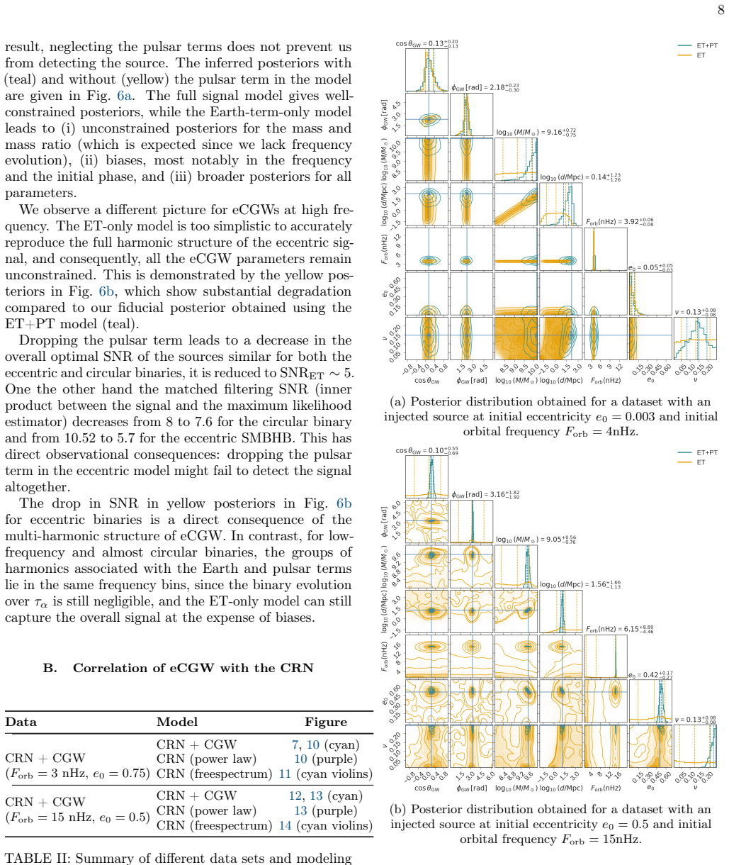
On the paper's own terms, the central discovery is that the degeneracy between total mass and mass ratio in a continuous-wave search is broken by eccentricity. For a high-frequency ($F_{\rm orb}\approx 15$ nHz) binary with initial eccentricity $e_0=0.5$, simulated six-pulsar data with white noise only yield informative posterior distributions for the symmetric mass ratio $\nu$, and therefore for $m_1$ and $m_2$, when the waveform includes both Earth and pulsar terms and post-leading-order post-Newtonian dynamics. The same data fitted with leading-order dynamics produce broader, biased posteriors, and with pulsar-distance uncertainty $\sigma_{\rm pdist}=5\%$ the injected $m_2$ falls outside the $90\%$ credible interval. Fitting with the Earth term only leaves all eccentric-CGW parameters unconstrained at high frequency, because the pulsar term is what carries the frequency-evolution information. At low frequency and low eccentricity ($F_{\rm orb}\approx 4$ nHz, $e_0\approx 0.003$), the binary hardly evolves over the pulsar light-travel time, so the Earth-term-only model still detects the signal but cannot constrain mass or distance. The paper also establishes a correlation between the eccentric continuous-wave signal and common red noise at low frequencies: a highly eccentric $3$ nHz binary produces a broad harmonic spectrum that the common red noise can partially absorb, yielding a bimodal likelihood and a Bayes factor $B\approx 0.7$ against the signal model, even though per-parameter prior-posterior distance metrics show that the data are informative.
Load-bearing premise
The load-bearing premise is that the post-leading-order eccentric binary evolution model from the authors' earlier paper faithfully describes the real orbital dynamics over the pulsar light-travel time; the mass measurement is extracted from that model's predicted frequency and eccentricity evolution, and the same model both generates and fits the simulated data.
Editorial extensions
If this is right
- A detected eccentric supermassive black hole binary at tens of nanohertz yields individual masses, not just a chirp mass, turning pulsar timing arrays into instruments for dynamical mass measurement of supermassive black holes.
- The pulsar term is not optional at high frequency: dropping it halves the matched-filter SNR from 10.52 to 5.7 for the shown eccentric source and leaves parameters unconstrained, so eccentric-search pipelines must include it.
- Using leading-order orbital dynamics for high-frequency sources biases $m_1$ and $m_2$ outside the $90\%$ credible interval when pulsar distances are known to $5\%$, so higher-order post-Newtonian evolution is required for unbiased masses.
- Tighter pulsar-distance priors, from $20\%$ to $5\%$, mainly sharpen sky localisation rather than the binary parameters, identifying distance knowledge as the current limit on source position.
- Low-frequency eccentric sources can be partially absorbed by the common red noise; a Bayes factor near unity does not mean the signal is absent, and per-parameter prior-posterior distances are a useful complementary diagnostic.
Reading between the lines
- If pulsar timing arrays detect a handful of high-frequency eccentric binaries, the individual-mass measurements could yield a direct dynamical census of supermassive black hole masses that bypasses scaling relations used in population studies.
- The bimodal likelihood and near-unity Bayes factor imply that global model selection may miss low-frequency eccentric continuous-wave candidates; targeted searches with external priors, for example from galaxy catalogues, could break the degeneracy with the background.
- The mass-measurement claim is only as strong as the orbital-evolution model used to generate the pulsar term; an independent cross-validation of that model against a differently implemented waveform, or against a real detection with an independent mass measurement, would be the natural next test.
- The GPU-accelerated likelihood makes joint background-plus-source searches at full array scale computationally feasible, so the same methodology can be applied to the next generation of pulsar timing data sets.
Editorial analysis
A structured set of objections, weighed in public.
Referee Report
Summary. This paper presents Bayesian injection-recovery studies for continuous gravitational-wave signals from eccentric supermassive-black-hole binaries in simulated PTA datasets. The signal model is the authors' earlier post-leading-order eccentric waveform [9], and the main scientific claims are (i) individual component masses can be measured when the source is at high orbital frequency, provided both the pulsar term and post-leading-order PN dynamics are included; (ii) dropping the pulsar term or truncating the dynamics to leading order degrades or biases the recovered parameters; and (iii) at low frequencies an eccentric CGW can be partially absorbed by a common red-noise process, giving a bimodal posterior and a Bayes factor of order unity. The paper also reports a GPU-compatible implementation and downsampling tests.
Significance. Within the self-consistency of the adopted waveform, this is a substantial and useful parameter-estimation study. The demonstration that the pulsar term and high-order PN evolution can break the mass-ratio degeneracy is physically well motivated, and the honest reporting of near-unity Bayes factors and the prior-volume penalty is a strength. The CRN-eCGW degeneracy and its impact on model selection are important for real PTA analyses. However, the physical significance of the headline mass-measurement claim is currently conditional on the fidelity of the authors' own waveform model [9], which is not independently validated in this manuscript.
major comments (2)
- [Sec. IVA, Eqs. (4)-(5), ref. [9]] The headline claim that the symmetric mass ratio ν and hence m1 and m2 are measurable is established only within the authors' own post-leading-order eccentric waveform model. The simulated residuals are generated with the same dynamical equations and harmonic amplitudes used for recovery, so the injection-recovery tests demonstrate pipeline self-consistency but not the physical fidelity of the waveform. In particular, the leading-order-model biases shown in Figs. 2-3 are measured against the same higher-order model used to make the injections, not against an independent truth. The limitations subsection (Sec. V.c) does not list waveform fidelity as a limitation. To support the central claim, the authors should either cross-check [9] against an independent eccentric waveform implementation, for example another PN code or established 2PN/3PN results, and examine sensitivity to unmodeled effects such as spins, or explicitly reframe the result as a pipeline demonstration conditional on [9].
- [Sec. V.c vs. Sec. IVB, Figs. 7, 10] The limitation paragraph states 'we fix the CRN and WN parameters,' but the low-frequency CRN+CGW analysis in Sec. IVB explicitly says 'We infer the parameters of the eccentric SMBHB together with the CRN parameters,' and Fig. 10 presents posterior distributions for log10 A_CRN and γ_CRN. This contradiction is not cosmetic: whether the CRN is fitted or fixed changes the meaning of the bimodal likelihood, the CRN-only comparison, and the reported Bayes factor. Please correct the limitation statement and make clear in Table II which parameters were held fixed in each run.
minor comments (6)
- [Table I and Sec. IVA/Conclusion] The low-frequency, near-circular injection is given as Forb = 4 nHz and e0 = 0.003 in the text and Fig. 5, but as Forb = 5 nHz and e0 = 0.01 in Table I and in Sec. V. Please harmonize these values.
- [Sec. IVB] The text refers to 'the EPTA DR2new dataset [9]', but reference [9] is the authors' waveform paper; the EPTA data papers should be cited instead.
- [Figs. 11 and 14] The Fig. 11 caption describes the free spectrum for the 'high frequency' dataset, but this figure appears in the low-frequency subsection and Fig. 14 is the high-frequency analogue; please check that the captions and table references are not swapped.
- [Throughout] There are several typographical and consistency issues that should be cleaned up: 'correponding', 'obtaine', 'Shanon', 'One the other hand', and 'Forb = 15,10nHz' in Sec. V.
- [Sec. IVA, Fig. 6] The comparison of posteriors with and without the pulsar term would be easier to assess if quantitative summaries, such as credible-interval widths or prior-posterior distances, were reported in addition to the corner plots.
- [Abstract and Sec. I] The abstract says the paper focuses on the 'detection strategy' for individual binaries, while Sec. I states that detectability is not considered and will be the subject of a separate publication; consider aligning the wording.
Circularity Check
Mass-measurement demonstration uses the authors' own [9] waveform both to inject and to recover the signal; the physical claim therefore rests on an uncross-checked self-citation, though the inference computations themselves are genuine.
-
self citation load bearing
[Section IVA (data model and mass estimation); Section V.a (conclusion)]
"We inject eCGW containing both Earth and pulsar terms at the highest PN order described in [9]. ... For the inference we are using several models: (i) eCGW model the same as injected, (ii) eCGW at leading order approximation, neglecting all high (post-leading order) PN corrections, (iii) eCGW with the Earth term only."
The headline claim that individual masses can be measured is demonstrated by simulating data with the authors' own [9] waveform and then fitting with that same waveform. The recovered unbiased masses are therefore a self-consistency property of the [9] model rather than an independent validation: any systematic error in the [9] dynamics would be invisible because the same equations generate the data and the likelihood. The conclusion then states 'Our results confirm the conjecture put forward in [9]', but the confirmation is internal to [9]'s framework and no independent waveform implementation is cross-checked. The physical mass-measurement claim thus reduces to the unverified self-citation [9] rather than to an externally anchored result.
full rationale
The paper is a careful injection-recovery study and most of its content is not circular: the Bayesian likelihood, the CRN/eCGW correlation analysis, the free-spectrum reconstructions, and the GPU implementation are genuine computations, and no parameter is fitted and then renamed a prediction. However, the central scientific claim in the abstract and conclusion -- that individual component masses can be measured from high-frequency eccentric PTA signals -- is built on the authors' prior waveform model [9] without independent cross-validation. Because the simulated datasets are generated with that same model and the 'correct' recovery model is that same model, the demonstrated unbiased recovery is a Monte-Carlo self-consistency check: it confirms the inference pipeline and the model's internal identifiability, but it cannot confirm the physical fidelity of [9]. The conclusion explicitly labels this as confirming the conjecture of [9], making the self-citation load-bearing for the headline claim. This warrants a moderate circularity score. The CRN-related results and the pulsar-distance study do not exhibit circularity.
Assumptions & free parameters
free parameters (5)
- Injected CRN amplitude =
log10 A_CRN = -14.5
- Injected CRN spectral index =
gamma_CRN = 4.33
- Posterior mode split threshold =
L_th = 537255.3
- Injected high-frequency eCGW parameters =
e0=0.5, Forb=14.85 nHz, log10 M=9.2, log10 d=1.2
- Free-spectrum Fourier components =
30
assumptions (4)
- domain assumption The eccentric binary waveform and post-leading-order PN dynamics of [9] faithfully describe SMBHB gravitational-wave emission.
- domain assumption The SGWB is adequately represented by a common uncorrelated red noise for studying CGW-noise degeneracy.
- standard math Timing residuals are Gaussian with a linearized timing model, and noise is stationary with power-law PSDs.
- domain assumption Pulsar distances are known to 20 percent (or 5 percent) relative Gaussian accuracy.
Cite this review
Pith. "Pith review of Parameter Estimation for Eccentric Supermassive Black Hole Binaries with Pulsar Timing Arrays." pith.science (2026). https://pith.science/paper/6CZGBY6X
@misc{pith2026260806944,
  author       = {Pith},
  title        = {Pith review of: Parameter Estimation for Eccentric Supermassive Black Hole Binaries with Pulsar Timing Arrays},
  year         = {2026},
  howpublished = {\url{https://pith.science/paper/6CZGBY6X}},
  note         = {Machine review of arXiv:2608.06944}
}
read the original abstract
Pulsar timing array (PTA) experiments are searching for gravitational waves (GWs) in the nanohertz band. The primary GW sources targeted by PTAs include populations of inspiralling supermassive black hole binaries (SMBHBs) in the local Universe, some of which may emit detectable continuous gravitational-wave (CGW) signals. In this paper, we focus on the detection strategy for individual binaries on eccentric orbits. Using simulated datasets based on the EPTA DR2new configuration, we perform injection-recovery studies across the parameter space. We demonstrate that individual component masses can be measured when an eccentric SMBHB is detected at high GW frequencies. We further show a correlation between the CGW signal and the stochastic gravitational-wave background (SGWB) at low frequencies, which makes CGW identification challenging. Finally, the developed software is GPU-compatible, enabling efficient Bayesian inference. This work lays the groundwork for future applications to real PTA data.
Figures


Figures from the paper (11 more)



Reference graph
Works this paper leans on
-
[9]
D. J. Reardonet al., Astrophys. J. Lett.951, L6 (2023), arXiv:2306.16215 [astro-ph.HE]
arXiv 2023
-
[1]
Frequency Domain Likelihood We can compute the likelihood more efficiently by ap- proximating the CRN as [16, 17]: Σα =N α +F αΦFT α ,(12) where Fα = {sinω itα,cosω itα} are the partial Fourier basis functions andΦij = S(fi)δij/T, assuming that the frequencies are uncorrelated.1 The inversion of this covariance matrix can be per- formed efficiently using ...
-
[2]
The first is the computation ofCij(τ )from Eq
Time-Domain Likelihood The likelihood can be evaluated in the time domain; however, this approach involves two computationally ex- pensive steps. The first is the computation ofCij(τ )from Eq. (9) and the inversion of the full covariance matrix Σ−1 α , which constitutes the main computational bottle- neck. The second is the evaluation of the eCGW template...
-
[3]
Posteriors We infer the posterior distribution of the data-model parameters (eCGW and noise) within a Bayesian frame- work: p(Θ, λ|δt,Ma) = L(δt|Θ, λ,Ma)π(Θ, λ|Ma) p(δt|Ma) .(15) Here, Ma denotes the assumed data model, where we separate the parameters describing the eCGW signal (Θ) from those describing the noise (λ). The prior distribution of these para...
-
[4]
J. P. W. Verbiestet al., Mon. Not. Roy. Astron. Soc.458, 1267 (2016), arXiv:1602.03640 [astro-ph.IM]
arXiv 2016
-
[5]
L. Z.Kelley, Z.Haiman, A. Sesana,and L. Hernquist, Mon. Not. Roy. Astron. Soc.485, 1579 (2019), arXiv:1809.02138 [astro-ph.HE]
arXiv 2019
-
[6]
J. Antoniadiset al. (EPTA, InPTA), Astron. Astrophys. 678, A50 (2023), arXiv:2306.16214 [astro-ph.HE]
arXiv 2023
-
[7]
G. Agazieet al. (NANOGrav), Astrophys. J. Lett.951, L8 (2023), arXiv:2306.16213 [astro-ph.HE]
arXiv 2023
Show all 35 references
-
[8]
curse of dimensionality
The residuals and the spectrum of harmonics for this source are presented in Fig. 5. This binary does not evolve significantly overτα, for example, for pulsar J1744-1134, the eccentricity at the pulsar term isep 0 = 0.004, and the orbital frequency isF p orb = 3.16nHz. As a 8 ...
-
[10]
Vallisneri, M
M. Vallisneri, M. Crisostomi, A. D. Johnson, and P. M. Meyers, Phys. Rev. Lett.135, 071401 (2025), arXiv:2405.08857 [gr-qc]
2025 arXiv
-
[11]
P. A. Rosado, A. Sesana, and J. Gair, Mon. Not. Roy. Astron. Soc.451, 2417 (2015), arXiv:1503.04803 [astro- ph.HE]
2015 arXiv
-
[12]
R. J. Truant, D. Izquierdo-Villalba, A. Sesana, G. M. Shaifullah, and M. Bonetti, Astron. Astrophys.694, A282 (2025), arXiv:2407.12078 [astro-ph.GA]
2025 arXiv
-
[13]
R. J. Truant, D. Izquierdo-Villalba, A. Sesana, G. M. Shaifullah, M. Bonetti, D. Spinoso, and S. Bonoli, Astron. Astrophys.706, A115 (2026), arXiv:2504.01074 [astro- ph.GA]
2026 arXiv
-
[14]
Manzini and S
S. Manzini and S. Babak, Phys. Rev. D114, 024036 (2026), arXiv:2511.19611 [gr-qc]
2026
-
[15]
Lentatiet al., Mon
L. Lentatiet al., Mon. Not. Roy. Astron. Soc.458, 2161 (2016), arXiv:1602.05570 [astro-ph.IM]
2016 arXiv
-
[16]
van Haasteren and Y
R. van Haasteren and Y. Levin, Mon. Not. Roy. Astron. Soc.428, 1147 (2013), arXiv:1202.5932 [astro-ph.IM]
2013 arXiv
-
[17]
Chalumeau et al
A. Chalumeau et al. (EPTA), Mon. Not. Roy. Astron. Soc.509, 5538 (2021), arXiv:2111.05186 [astro-ph.HE]
2021 arXiv
-
[18]
R. W. Hellings and G. S. Downs, Astrophys. J. Lett.265, L39 (1983)
1983
-
[19]
Discovery, Discovery: next-generation pulsar-timing-array data-analysis package, built for speed on a jax back- end that supports gpu execution and autodifferentiation, https://github.com/nanograv/discovery(2025)
2025
-
[20]
Lentati, P
L. Lentati, P. Alexander, M. P. Hobson, S. Taylor, J. Gair, S. T. Balan, and R. van Haasteren, Phys. Rev. D87, 104021 (2013), arXiv:1210.3578 [astro-ph.IM]
2013 arXiv
-
[21]
van Haasteren and M
R. van Haasteren and M. Vallisneri, Phys. Rev. D90, 104012 (2014), arXiv:1407.1838 [gr-qc]
2014 arXiv
-
[22]
Crisostomi, R
M. Crisostomi, R. van Haasteren, P. M. Meyers, and M. Vallisneri, Beyond diagonal approximations: improved covariance modeling for pulsar timing array data analysis (2025), arXiv:2506.13866 [astro-ph.IM]
2025 arXiv
-
[23]
Karnesis, M
N. Karnesis, M. L. Katz, N. Korsakova, J. R. Gair, and N. Stergioulas, Mon. Not. Roy. Astron. Soc.526, 4814 (2023), arXiv:2303.02164 [astro-ph.IM]
2023 arXiv
-
[24]
Ivezić, A
Ž. Ivezić, A. J. Connolly, J. T. VanderPlas, and A. Gray, Statistics, Data Mining, and Machine Learning in Astronomy (Princeton University Press, 2014)
2014
-
[25]
Skilling, AIP Conf
J. Skilling, AIP Conf. Proc.735, 395 (2004)
2004
-
[26]
T. B. Littenberg and N. J. Cornish, Phys. Rev. D107, 063004 (2023), arXiv:2301.03673 [gr-qc]
2023 arXiv
-
[27]
Speri, N
L. Speri, N. K. Porayko, M. Falxa, S. Chen, J. R. Gair, A. Sesana, and S. R. Taylor, Mon. Not. Roy. Astron. Soc. 518, 1802 (2022), arXiv:2211.03201 [astro-ph.HE]
2022 arXiv
-
[28]
S. Hee, W. Handley, M. P. Hobson, and A. N. Lasenby, Mon. Not. Roy. Astron. Soc.455, 2461 (2016), arXiv:1506.09024 [astro-ph.CO]
2016 arXiv
-
[29]
Bartolucci, L
F. Bartolucci, L. Scaccia, and A. Mira, Biometrika93, 41 (2006)
2006
-
[30]
We define these two metrics in the Appendix A
and Jensen-Shannon [31] marginalised per-parameter distances between the posteriors p(Θi)and the priors π(Θi)for the full WN+CRN+eCGW runs at low and high frequency. We define these two metrics in the Appendix A. The per-parameter metrics for the eCGW parameters of both binari...
-
[31]
Chenet al
S. Chenet al. (EPTA), Mon. Not. Roy. Astron. Soc.508, 4970 (2021), arXiv:2110.13184 [astro-ph.HE]
2021 arXiv
-
[32]
Antoniadiset al
J. Antoniadiset al. (EPTA), Astron. Astrophys.678, A48 (2023), arXiv:2306.16224 [astro-ph.HE]
2023 arXiv
-
[33]
Korsakova, S
N. Korsakova, S. Babak, M. L. Katz, N. Karnesis, S. Khukhlaev, and J. R. Gair, Phys. Rev. D110, 104069 (2024), arXiv:2402.13701 [gr-qc]
2024 arXiv
-
[34]
Bhattacharyya, Bull
A. Bhattacharyya, Bull. Calcutta Math. Soc.35, 99 (1943)
1943
-
[35]
Lin, IEEE Trans
J. Lin, IEEE Trans. Info. Theor.37, 145 (1991)
1991
Reviewed August 10, 2026 · model on record in the stance chip above.
Discussion (0). Continue with ORCID to comment.