REVIEW 3 major objections 5 minor 32 references
The traveling wave solutions of the 1D hyperbolic Keller-Segel equations
T0 review · 3 major / 5 minor · reviewed 2026-08-16 · deepseek-v4-flash
Pith's one-line read The 1D hyperbolic Keller-Segel system admits entropy-admissible traveling waves for every speed; non-vacuum profiles are necessarily continuous.
desk verdict The vacuum half of this paper is new and sound; the non-vacuum half, as written, rests on a false inequality that leaves Theorem 1.2's main clause unproved, though the flaw is local and fixable. read the letter →
The pith
A machine-rendered reading of the paper's core claim, the machinery that carries it, and where it could break.
The reading
What carries the argument
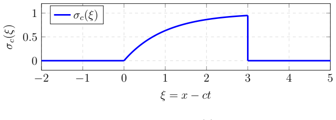
The organizing object is the reduced profile system obtained in the moving frame $\xi=x-ct$. Integrating the first PDE once and using the far-field condition fixes a flux constant: in the vacuum case the zero-flux relation $-c\sigma_c+\sigma_c(1-\sigma_c)\partial_\xi S_c=0$, and in the non-vacuum case equation (5.13). On any interval where $\sigma_c>0$ this relation expresses $\sigma_c$ algebraically in terms of $\partial_\xi S_c$, converting the PDE pair into a two-dimensional ODE system for $(S_c,\partial_\xi S_c)$; the entropy inequality supplies Rankine-Hugoniot conditions (2.8)-(2.10) that select admissible jumps. For the non-vacuum case the algebraic relation is a quadratic, $p(x)=0$, and the proof of continuity rests on the fact that $p(\sigma_\infty)<0$, so the two possible values at a jump would straddle $\sigma_\infty$ and force a sign change in $\partial_\xi S_c$, violating the entropy condition.
What would settle it
Numerically shoot the non-vacuum profile equations with far-field data $\sigma(-\infty)=\sigma_\infty$, $S(-\infty)=\sigma_\infty$, but $\partial_\xi S(-\infty)=\delta\neq 0$: any bounded entropy-admissible solution of (1.1) found this way would lie outside the four families of Propositions 5.7-5.10 and would refute exhaustiveness of the classification.
Extended reading notes
Core claim
The paper's central claim is Theorem 1.2: for every $c\in\mathbb{R}$ there exist traveling wave solutions $\sigma(t,x)=\sigma_c(x-ct)$, $S(t,x)=S_c(x-ct)$ of system (1.1) satisfying the entropy inequality (2.4), with either vacuum far field (1.2) or non-vacuum far field (1.3). In the vacuum case the classification gives continuous right-going and left-going profiles as well as profiles with a single jump, with the entropy condition permitting a jump only between a vacuum state and a non-vacuum state and fixing the required sign of the speed. In the non-vacuum case, for $\sigma_\infty\in(0,1)$, Propositions 5.6 through 5.10 show that every non-trivial traveling profile is continuous, never touches the far-field value except at infinity, and belongs to one of four families determined by the sign of $c$ and whether $\sigma_c$ stays above or below $\sigma_\infty$. A companion classification of stationary solutions gives one-parameter families with a single jump. The paper's stated conclusion is that these results provide explicit examples of the non-uniqueness of entropy-admissible weak solutions and highlight the limitations of the entropy condition as a selection criterion.
Load-bearing premise
The load-bearing assumption is that the profile reaches its far-field equilibrium with $\partial_\xi S_c\to 0$, because that is what fixes the integration constant; if a bounded front approaches infinity with a non-vanishing or oscillatory derivative, the classification need not be exhaustive.
Editorial extensions
If this is right
- For every speed $c$ there is an explicit global weak solution to (1.1), so the entropy-admissible solution set is non-empty beyond the stationary states.
- With vacuum far field, entropy permits both continuous and single-jump traveling waves; the jump must connect vacuum to a non-vacuum state, with $c<0$ for a vacuum-to-active jump and $c>0$ for an active-to-vacuum jump.
- With non-vacuum far field in $(0,1)$, no entropy-admissible traveling wave can carry a shock; any moving discontinuity would have to connect states on opposite sides of $\sigma_\infty$, which contradicts the jump sign condition.
- The stationary classification includes one-parameter families of piecewise smooth solutions, giving further concrete instances where the entropy inequality fails to single out a unique weak solution.
- The saturated case $\sigma_\infty=1$ is reduced to the vacuum case by the change of variables $\eta=1-\sigma$, $Q=1-S$.
Reading between the lines
- If the one-sided semi-wave convention were replaced by a two-sided far-field condition, the integration constant in the flux relation would generally be nonzero; the classification would likely become a family parameterized by that constant, and shocks connecting non-vacuum states might reappear.
- The non-vacuum no-jump result suggests that, for initial data near a non-vacuum equilibrium, shocks formed dynamically by the Burgers-type nonlinearity cannot asymptotically persist as traveling discontinuities; they must either be smoothed out or leave the observable profile.
- A natural next step is a stability analysis of these explicit profiles; the exponential asymptotics in Propositions 5.7-5.10 give concrete linearized operators for such a study.
- One could test exhaustiveness numerically by shooting from the far field with a modified boundary condition on $\partial_\xi S_c$; a bounded entropy-admissible profile found there would lie outside the stated classification.
Signed reviews
Editorial analysis
A structured set of objections, weighed in public.
Referee Report
Summary. The paper constructs stationary and traveling wave solutions for the one-dimensional hyperbolic Keller-Segel system with quorum sensitivity, under one-sided far-field conditions. For the vacuum far-field case it classifies stationary profiles and builds both continuous and single-jump traveling waves for c>0 and c<0. For the non-vacuum far-field case, after reducing σ∞=1 by symmetry, it claims that all nontrivial traveling profiles are continuous and characterizes them by four families. The intended contribution is to exhibit explicit entropy-admissible weak solutions and thereby show that the entropy condition alone does not select uniqueness. The stationary and vacuum sections are largely self-contained and explicit, with jump conditions checked by hand. The non-vacuum construction, however, rests on a comparison estimate, Eq. (5.36), that is algebraically false, and the claimed global exponential bounds in Propositions 5.7–5.10 are therefore unsupported. The proof of the entropy jump condition in Proposition 2.1 is also circular as written.
Significance. If the non-vacuum part were correctly proved, the paper would give a valuable explicit family of entropy-admissible weak solutions, including piecewise smooth profiles, and would provide a clean demonstration that the entropy inequality (2.4) is not a uniqueness selection criterion. The stationary and vacuum traveling-wave constructions are explicit, parameterized by A0, c, and σ∞, and the entropy checks for those jumps are concrete and verifiable. These parts represent a solid contribution. However, the main theorem’s non-vacuum clause is load-bearing for the paper’s central claim, and that clause is not established as printed because Eq. (5.36) is false and because the proof of Proposition 2.1 is circular. The defect is local and appears fixable in principle, but it is not a presentational issue: it directly invalidates the derivation of (5.37) and hence the asserted asymptotics and global existence in Propositions 5.7–5.10.
major comments (3)
- [§5.3.1, Eq. (5.36)] Equation (5.36) is false. With V=Tc+Rc/(2c), equation (5.35) gives ∂ξV=Rc+αTc with α=1/(2c)−σc(1−σc)/c ∈ [1/(4c), 1/(2c)). The claimed lower bound (1/(4c)+2c)V ≤ ∂ξV would require Rc(1−(1/(4c)+2c)/(2c)) + Tc(α−(1/(4c)+2c)) ≥ 0. Since (1/(4c)+2c)/(2c) = 1/(8c^2)+1 > 1, the coefficient of Rc is negative, so the inequality fails whenever Rc is large relative to Tc. For example, c=0.1, Rc=1, Tc=0.01 satisfy (5.35) but give ∂ξV ≈ 1.025–1.05, whereas (1/(4c)+2c)V ≈ 13.5. Consequently the exponential bounds (5.37) are unsupported. Since Proposition 5.7 items 2–3 use (5.37) for global existence and asymptotics, and since Propositions 5.8–5.10 say the proof follows by analogous comparison arguments, the non-vacuum half of Theorem 1.2 is not proved as written. A correct lower comparison coefficient would have to be of the form min(2c, 1/(4c)) (or arise from a different c-dependent estimate), not the sum 2c+1/(4c).
- [§2, Proposition 2.1] The proof of Proposition 2.1 is circular. After deriving the Rankine–Hugoniot relations (2.14)–(2.16), the authors introduce Kružkov entropies and, in the case σ−≤σ0≤σ+, write “Thus (2.10) implies (2.19)” and similarly in the reverse case. But (2.10) is exactly the statement being proved. The entropy inequality (2.16) should be used to derive (2.19) and its counterpart; as printed, the key jump condition (2.10), which is used throughout Sections 3–5 to rule out discontinuities, is not established. This is a local but load-bearing gap in the admissibility verification.
- [§5.3.1, integral curve construction] The construction of the integral curve for (5.38) through (R++,Y++)=(0,0) is not fully justified. The right-hand side of (5.38) is not Lipschitz in Y at Y=0, because σc(√Y) has the expansion σ∞+c1√Y+o(√Y) with c1>0 by (5.39), so the Picard–Lindelöf theorem does not apply at the origin. The ε→0 limit and bootstrap give a solution, but the sentence “Thus one can conclude that (R++,Y++,0(R++)) is the unique integral curve for (5.38) passing through (R++,Y++)=(0,0)” does not follow from the displayed estimates; multiple tangent directions at the origin are not excluded. Since Proposition 5.7 item 1 asserts uniqueness of this curve, the non-vacuum classification needs an additional argument here.
minor comments (5)
- [§5.3.3 and §5.3.4] In Propositions 5.9 and 5.10, item 2 says the ODE system is “with (5.46)”, but for those cases the correct formulas are (5.51) and (5.56), respectively.
- [§4.3.1, after (4.67)] The sentence “for some 0<−2c<c1” is unclear; presumably a positive lower bound comparable to |c| was intended, and the notation should be made precise.
- [§5.3.1, after (5.37)] The phrase “provided that the solution to (5.30)” is an incomplete sentence; it should read “provided that the solution to (5.30) exists.”
- [§4.2.2, paragraph before Proposition 4.7] The argument that ξ2=∞ should state explicitly that continuity of Sc and Yc at ξ2 follows from (2.8); as written the contradiction in (4.53) is compressed and easy to misread.
- [§6 Conclusion] The phrase “complete classification” overstates what is proved: the theorems establish existence of explicit families, and for the non-vacuum case the classification claim is conditional on Definition 4.1 and on the repairs described above. The wording of the conclusion should be aligned with the precise statements of Theorems 1.1–1.2.
Circularity Check
Only circular thread is a proof-direction slip in Proposition 2.1; the traveling-wave constructions themselves are self-contained and do not reduce to fitted inputs.
-
other
[Section 2, proof of Proposition 2.1, Eqs. (2.18)–(2.20)]
"Thus (2.10) implies ∂xS(σ0−σ+)(σ0−σ−)≥0.(2.19) Similarly, for σ+≤σ0≤σ−, one has that ∂xS(σ0−σ+)(σ0−σ−)≤0.(2.20) This finishes the proof of Proposition 2.1."
Proposition 2.1 is supposed to derive the jump conditions, including the sign condition (2.10), from the entropy inequality (2.4)/(2.16). Instead, the proof inserts (2.10) itself as an assumption to obtain the intermediate inequalities (2.19)–(2.20), then immediately concludes. Thus the target condition (2.10) is assumed rather than shown to follow from the entropy inequality; no independent derivation of (2.10) from (2.16) is displayed. The surrounding algebra indicates the intended reverse implication, so this is a logical-direction slip rather than a deep circularity, but as printed it is a genuine instance of using the conclusion as an input.
full rationale
This is a pure PDE construction paper. No parameter is fitted to data, no output quantity is defined in terms of the claim being proved, and no load-bearing result is imported from a self-citation chain. The main traveling-wave constructions start from the ansatz (4.1), integrate (4.2a) to obtain the zero-flux relation (4.4), and solve the resulting first-order ODE systems independently of the theorems being asserted; the vacuum and non-vacuum classifications are obtained from those ODEs, not from the claimed existence. The one-sided far-field convention in Definition 4.1 is a stated modeling assumption that fixes the integration constant; it is not derived from, nor identical to, the claimed existence result, so it is not circular. The only circular-seeming passage is in the proof of Proposition 2.1, where the target sign condition (2.10) is used to verify (2.19)–(2.20) and the proof then stops. Because the reverse implication from the entropy inequality (2.16) to (2.10) is elementary and the rest of the paper's profile constructions do not depend numerically on this slip, this is a presentation-level logical inversion rather than substantive circularity. The algebraic defect in (5.36) identified by the reviewer is a correctness concern, not a circularity, and is therefore not counted in this score.
Assumptions & free parameters
free parameters (5)
- A0
- c
- σ∞
- A
- R++ and analogous R+-, R-+, R--
assumptions (4)
- standard math Weak solutions and Kružkov entropy pairs are used as the admissibility framework; the entropy inequality (2.4) is imposed at shocks.
- standard math For σ∈L∞, the elliptic equation -S''+S=σ has S∈W^{2,p} with S and S' continuous, so [[S]]=[[S']]=0 holds at jumps.
- standard math Picard-Lindelöf existence, Gronwall's inequality, and Arzela-Ascoli compactness justify the ODE constructions and the integral-curve limits in Sections 4 and 5.
- domain assumption The one-sided far-field convention permits profiles whose second equilibrium is replaced by unbounded growth or decay of S at the opposite infinity.
Cite this review
Pith. "Pith review of The traveling wave solutions of the 1D hyperbolic Keller-Segel equations." pith.science (2026). https://pith.science/paper/IS56FTXH
@misc{pith2026260812226,
  author       = {Pith},
  title        = {Pith review of: The traveling wave solutions of the 1D hyperbolic Keller-Segel equations},
  year         = {2026},
  howpublished = {\url{https://pith.science/paper/IS56FTXH}},
  note         = {Machine review of arXiv:2608.12226}
}
read the original abstract
The goal of this paper is to investigate the traveling wave solutions with one-sided far field conditions for the one-dimensional hyperbolic Keller-Segel equations with quorum sensitivity. The traveling wave solutions are piece-wise smooth in the moving coordinate, and satisfy the entropy inequality at the discontinuity.
Figures


Figures from the paper (5 more)


Reference graph
Works this paper leans on
-
[1]
Stability and instability for the fully parabolic Keller-Segel system around constant equilibrium
Jaewook Ahn, Jae-Myoung Kim, and Junha Kim. Stability and instability for the fully parabolic Keller-Segel system around constant equilibrium, July 2026. arXiv:2607.10384 [math.AP]
work page Pith review arXiv 2026
-
[2]
On the blow-up profile of Keller–Segel–Patlak system
Xueli Bai and Maolin Zhou. On the blow-up profile of Keller–Segel–Patlak system. Mathematische Annalen, 392(1):313–337, May 2025
work page 2025
-
[3]
Carrillo, and Philippe Lauren¸ cot
Adrien Blanchet, Jos´ e A. Carrillo, and Philippe Lauren¸ cot. Critical mass for a Pat- lak–Keller–Segel model with degenerate diffusion in higher dimensions.Calculus of Variations and Partial Differential Equations, 35(2):133–168, June 2009
work page 2009
-
[4]
Adrien Blanchet, Jos´ e A. Carrillo, and Nader Masmoudi. Infinite time aggre- gation for the critical Patlak-Keller-Segel model in$\mathbb Rˆ2$.Commu- nications on Pure and Applied Mathematics, 61(10):1449–1481, 2008. eprint: https://onlinelibrary.wiley.com/doi/pdf/10.1002/cpa.20225
-
[5]
Adrien Blanchet, Jean Dolbeault, and Benoˆ ıt Perthame. Two-dimensional Keller-Segel model: Optimal critical mass and qualitative properties of the solutions.Electronic Journal of Differential Equations (EJDE) [electronic only], 2006:Paper No. 44, 33 p., electronic only–Paper No. 44, 33 p., electronic only, 2006. 30
work page 2006
-
[6]
F. Bouchut and B. Perthame. Kruzkov’s estimates for scalar conservation laws revisited. Transactions of the American Mathematical Society, 350(7):2847–2870, 1998
work page 1998
-
[7]
Myeongju Chae, Kyungkeun Kang, and Jihoon Lee. Existence of smooth solutions to coupled chemotaxis-fluid equations.Discrete and Continuous Dynamical Systems, 33(6):2271–2297, December 2012
work page 2012
-
[8]
Giani Ega˜ na Fern´ andez and St´ ephane Mischler. Uniqueness and Long Time Asymp- totic for the Keller–Segel Equation: The Parabolic–Elliptic Case.Archive for Rational Mechanics and Analysis, 220(3):1159–1194, June 2016
work page 2016
Show all 32 references
-
[9]
On convergence to equilibria for the Keller–Segel chemotaxis model.Journal of Differential Equations, 236(2):551– 569, May 2007
Eduard Feireisl, Philippe Lauren¸ cot, and Hana Petzeltov´ a. On convergence to equilibria for the Keller–Segel chemotaxis model.Journal of Differential Equations, 236(2):551– 569, May 2007
2007
-
[10]
Strong so- lutions to the Keller-Segel-Navier-Stokes system in bounded Lipschitz domains, May
Matthias Hieber, Hideo Kozono, Sylvie Monniaux, and Patrick Tolksdorf. Strong so- lutions to the Keller-Segel-Navier-Stokes system in bounded Lipschitz domains, May
-
[11]
Hillen and K
T. Hillen and K. J. Painter. A user’s guide to PDE models for chemotaxis.Journal of Mathematical Biology, 58(1):183–217, January 2009
2009
-
[12]
Nieders¨ achsische Staats- und Universit¨ atsbibliothek, 2003
Dirk Horstmann.From 1970 Until Present: the Keller-Segel Model in Chemotaxis and Its Consequences. Nieders¨ achsische Staats- und Universit¨ atsbibliothek, 2003. Google- Books-ID: SfL xwEACAAJ
1970
-
[13]
Long-time dynamics of classical Keller–Segel equation
Chia-Yu Hsieh and Yong Yu. Long-time dynamics of classical Keller–Segel equation. Nonlinear Analysis: Real World Applications, 76:104026, April 2024
2024
-
[14]
Keller and Lee A
Evelyn F. Keller and Lee A. Segel. Initiation of slime mold aggregation viewed as an instability.Journal of Theoretical Biology, 26(3):399–415, March 1970
1970
-
[15]
Existence and uniqueness theorem on weak solutions to the parabolic–elliptic Keller–Segel system.Journal of Differential Equations, 253(7):2295–2313, October 2012
Hideo Kozono, Yoshie Sugiyama, and Yumi Yahagi. Existence and uniqueness theorem on weak solutions to the parabolic–elliptic Keller–Segel system.Journal of Differential Equations, 253(7):2295–2313, October 2012
2012
-
[16]
S. N. Kruˇ zkov. FIRST ORDER QUASILINEAR EQUATIONS IN SEVERAL INDE- PENDENT VARIABLES.Mathematics of the USSR-Sbornik, 10(2):217, February 1970
1970
-
[17]
Threshold for shock formation in the hyperbolic Keller–Segel model.Applied Mathematics Letters, 50:56–63, December 2015
Yongki Lee and Hailiang Liu. Threshold for shock formation in the hyperbolic Keller–Segel model.Applied Mathematics Letters, 50:56–63, December 2015
2015
-
[18]
Finite time blowup for Keller-Segel equation with logistic damping in three dimensions, July 2025
Jiaqi Liu, Yixuan Wang, and Tao Zhou. Finite time blowup for Keller-Segel equation with logistic damping in three dimensions, July 2025. arXiv:2504.12231 [math]
2025 arXiv
-
[19]
Large friction limit of the almost pressureless Euler-Poisson system, March
Xin Liu. Large friction limit of the almost pressureless Euler-Poisson system, March
-
[20]
Global well-posedness, blow- up phenomenon and ill-posedness for the hyperbolic Keller-Segel equations.Journal of Differential Equations, 413:828–850, December 2024
Zhiying Meng, Yao Nie, Weikui Ye, and Zhaoyang Yin. Global well-posedness, blow- up phenomenon and ill-posedness for the hyperbolic Keller-Segel equations.Journal of Differential Equations, 413:828–850, December 2024
2024
-
[21]
Finite-time blow-up in hyperbolic Keller–Segel system of consumption type with logarithmic sensitivity.Nonlinearity, 37(4):045003, February 2024
Jungkyoung Na. Finite-time blow-up in hyperbolic Keller–Segel system of consumption type with logarithmic sensitivity.Nonlinearity, 37(4):045003, February 2024
2024
-
[22]
Global well-posedness for a two-dimensional Keller-Segel-Euler system of consumption type.Journal of Differential Equations, 388:188–214, April 2024
Jungkyoung Na. Global well-posedness for a two-dimensional Keller-Segel-Euler system of consumption type.Journal of Differential Equations, 388:188–214, April 2024
2024
-
[23]
Clifford S. Patlak. Random walk with persistence and external bias.The bulletin of mathematical biophysics, 15(3):311–338, September 1953
1953
-
[24]
Existence of Solutions of the Hyperbolic Keller-Segel Model.Transactions of the American Mathematical Society, 361(5):2319– 2335, 2009
Benoˆ ıt Perthame and Anne-Laure Dalibard. Existence of Solutions of the Hyperbolic Keller-Segel Model.Transactions of the American Mathematical Society, 361(5):2319– 2335, 2009
2009
-
[25]
Blow-up Profiles for the Parabolic–Elliptic Keller–Segel System in Dimensions$${n\geq 3}$$.Communications in Mathematical Physics, 367(2):665–681, April 2019
Philippe Souplet and Michael Winkler. Blow-up Profiles for the Parabolic–Elliptic Keller–Segel System in Dimensions$${n\geq 3}$$.Communications in Mathematical Physics, 367(2):665–681, April 2019
2019
-
[26]
Yoshie Sugiyama. Global existence in sub-critical cases and finite time blow-up in super- critical cases to degenerate Keller-Segel systems.Differential and Integral Equations, 19(8):841–876, January 2006
2006
-
[27]
Application of the best constant of the Sobolev inequality to degen- erate Keller-Segel models.Advances in Differential Equations, 12(2):121–144, January 2007
Yoshie Sugiyama. Application of the best constant of the Sobolev inequality to degen- erate Keller-Segel models.Advances in Differential Equations, 12(2):121–144, January 2007
2007
-
[28]
Time periodic strong solutions to the Keller-Segel sys- tem coupled to Navier-Stokes equation.Journal of Differential Equations, 298:95–131, October 2021
Zhong Tan and Zhonger Wu. Time periodic strong solutions to the Keller-Segel sys- tem coupled to Navier-Stokes equation.Journal of Differential Equations, 298:95–131, October 2021
2021
-
[29]
Michael Winkler. Global Large-Data Solutions in a Chemotaxis-(Navier–)Stokes System Modeling Cellular Swimming in Fluid Drops.Communications in Partial Differential Equations, 37(2):319–351, February 2012. eprint: https://doi.org/10.1080/03605302.2011.591865
2012
-
[30]
Stabilization in a two-dimensional chemotaxis-Navier–Stokes system
Michael Winkler. Stabilization in a two-dimensional chemotaxis-Navier–Stokes system. Archive for Rational Mechanics and Analysis, 211(2):455–487, February 2014. 32
2014
-
[2025]
arXiv:2505.04503 [math]
-
[2026]
arXiv:2603.18346 [math]. 31
Reviewed August 16, 2026 · model on record in the stance chip above.
Discussion (0). Continue with ORCID to comment.