REVIEW 3 major objections 6 minor 28 references
Monotonic and nonmonotonic immune responses in viral infection systems
T0 review · 3 major / 6 minor · reviewed 2026-08-14 · deepseek-v4-flash
Pith's one-line read The paper claims that nonmonotonic immune responses can make viral rebound and viral control both stable for the same parameters, while monotonic immune responses cannot.
desk verdict Solid but rough: the Monod-Haldane bistable interval is a real, explicitly computed result, yet the no-bistability wording outruns the proof and the manuscript needs revision before I would cite it. read the letter →
The pith
A machine-rendered reading of the paper's core claim, the machinery that carries it, and where it could break.
The reading
What carries the argument
The engine is the hump-shaped Monod-Haldane immune response $f(y)=cy/(\alpha+\gamma y+y^2)$. Because $f(y)$ rises to a peak and then falls, the balance equation $f(y)=b$ can have two positive roots $y_*^{2-}$ and $y_*^{2+}$ once $c>c_2$, and the sign of $\alpha-y^2$ decides which of these equilibria is stable and which is a saddle. The same nonmonotonic shape places the exchange of stability between the immune-free and immune-present equilibria at the transcritical threshold $c_1^{**}$ and the merging of the two positive equilibria at the saddle-node threshold $c_2$. Characteristic-equation stability analysis and the transversality conditions for bifurcations certify these transitions.
What would settle it
A concrete check: scan system (1.1) with a monotonic $f$ over the $b$–$p$ plane for two simultaneously stable equilibria, or continue periodic orbits numerically; finding a stable limit cycle coexisting with a stable equilibrium would show that the equilibrium-only version of Remark 2.1 leaves out an attractor, while finding two stable equilibria would refute it outright.
Extended reading notes
Core claim
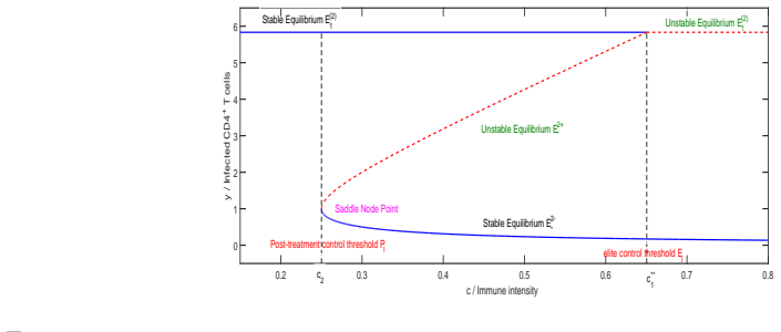
Consider system (1.3), where uninfected cells $x$, infected cells $y$, and immune cells $z$ evolve with immune growth $f(y)=cy/(\alpha+\gamma y+y^2)$. Under $\gamma>2\sqrt{\alpha}$ and $R_0^{(2)}>R_c^{(1)}>1$, the paper shows that for $c_2<c<c_1^{**}$ the immune-free equilibrium $E_1^{(2)}$ and the positive equilibrium $E_2^{*-}$ are simultaneously locally asymptotically stable, while $E_2^{*+}$ is a saddle: this is the bistable interval. Here $c_2=\gamma b+2b\sqrt{\alpha}$ is the post-treatment control threshold below which the immune-free state is the only stable outcome, and $c_1^{**}$ is the elite control threshold above which the positive equilibrium is the only stable outcome. The 2D analog (5.1) has the same threshold structure with its own elite threshold. For the monotonic systems (1.1) and (4.1), where $f'(y)>0$, the equilibria are stable in mutually exclusive regimes, so the paper concludes that bistability does not occur.
Load-bearing premise
The no-bistability conclusion for the monotonic systems assumes that 'bistability' means two stable steady states; if repeating cycles count as states, the 3D monotonic case is not settled, because Theorems 2.1–2.3 do not rule out stable oscillations.
Editorial extensions
If this is right
- In the nonmonotonic model, immune intensity below $c_2$ leaves only the immune-free equilibrium stable, so the virus rebounds after treatment.
- Above $c_1^{**}$ only the immune-present equilibrium is stable, so the virus stays under control.
- In the bistable interval $(c_2,c_1^{**})$, two stable outcomes coexist, so the same host parameters can produce either rebound or control depending on the initial infection load.
- The saddle-node at $c_2$ and the transcritical at $c_1^{**}$ are the organizing events through which the stable and unstable equilibria appear and disappear as immune intensity $c$ varies.
- For the monotonic systems, no two stable equilibria coexist, so each parameter regime has a single eventual outcome.
Reading between the lines
- If the threshold picture transfers to therapy, a patient whose immune intensity lies in the bistable interval should be pushed above $c_1^{**}$ by a temporary boost to immune stimulation; the paper does not model treatment, so this is an extrapolation.
- Because the 3D monotonic analysis proves local stability and one global result but does not rule out stable limit cycles, a broader definition of bistability that counts oscillatory attractors might still allow bistability in monotonic systems; that question is not settled here.
- The hump-shaped mechanism depends only on the shape of $f(y)$, so the same threshold structure may appear in other within-host infections whenever immune stimulation falls off at high viral load; the paper itself only analyzes the specific model families.
Signed reviews
Editorial analysis
A structured set of objections, weighed in public.
Referee Report
Summary. The paper analyzes four ODE models of viral infection with immune response: a 3D model and a 2D model, each with a monotone immune response, and corresponding versions with a nonmonotone Monod-Haldane immune response. For the monotone models the authors prove local stability of the equilibria and assert that no bistability occurs. For the nonmonotone models they derive two thresholds, the post-treatment control threshold c2 and the elite control threshold c**1 (or c**2), and prove that for immune intensity between these thresholds the system has two stable equilibria. They also apply Sotomayor's theorem to establish saddle-node bifurcation at c2 and transcritical bifurcation at the elite control threshold, and they support the analytical results with numerical simulations.
Significance. The proposed contrast between monotone and nonmonotone immune responses as a mechanism for bistability is biologically relevant and gives a clean mechanistic interpretation of post-treatment control versus viral rebound. A notable strength is that the thresholds are derived from the model parameters rather than fitted to data, and the 2D no-bistability statements are backed by Dulac's criterion, which excludes limit cycles. The bifurcation computations are explicit and checkable. The main limitation is that the corresponding no-bistability statements for the 3D systems are not global and therefore overstate the proved results if periodic attractors are admitted.
major comments (3)
- [Remarks 2.1 and 3.1; Theorems 2.1–2.3 and 3.2–3.4] The categorical statements that the 3D monotone system (1.1) and the 3D nonmonotone system (1.3) have no bistability outside the bistable interval are supported only by local stability analysis of equilibria. Theorems 2.1–2.3 and 3.2–3.4 show, at most, that no two stable equilibria coexist; they do not rule out stable limit cycles in R3, so coexistence of a stable equilibrium with a stable periodic orbit is not excluded. If the authors intend bistability to mean coexistence of two stable equilibria, that definition should be stated explicitly and the remarks restricted accordingly; otherwise the claims overstate what is proved.
- [Theorem 5.3, Section 5.1] The proof of Theorem 5.3 contains a sign error: it states that the eigenvalue λ2 = cy1/(α+γy1+y1^2) − b satisfies λ2 > 0 for 0 < c < c**2, but this eigenvalue is in fact negative exactly when c < c**2. Since the theorem's conclusion that E(4)_1 is locally and globally stable requires λ2 < 0, the proof as written contradicts its own assertion and must be corrected.
- [Theorems 3.6 and 5.6, transcritical bifurcation] The transcritical bifurcation proofs apply Sotomayor's theorem but do not verify the nondegeneracy conditions in the exceptional case R0 = Rc. At this parameter point y1 = √α, so α − y1^2 = 0, which makes the Sotomayor coefficient Γ3 (resp. Φ3) zero; in the 3D case c[tc] then coincides with c2 = c[sn], so the two bifurcations collide and the bifurcation is degenerate. The theorems state only R0 > 1 and c = c[tc], so this case is included; the authors should either exclude R0 = Rc or analyze the degenerate case separately.
minor comments (6)
- [Section 3.4 and Section 5.3] The transcritical-bifurcation theorem is numbered Theorem 5.6 in both sections; the theorem in Section 3.4 should be renumbered Theorem 3.6.
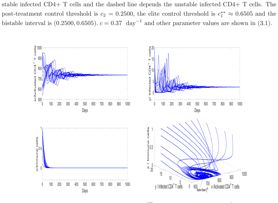
- [Figure 1 caption and Section 3.5] Figure 1 reports c2 = 0.2500 and c**1 ≈ 0.6505, whereas the text for the same parameter set (3.1) gives c2 = 0.3000 and c**1 ≈ 0.3837; the caption and text should be reconciled.
- [Section 5.4] The text states that the bistable interval is (2.5000, 3.8333), but the computed value c**2 ≈ 3.5278 and the caption of Figure 5 give (2.5000, 3.5278); the numbers should be made consistent.
- [Section 5.4, parameter list] The parameter list uses the symbol γ twice (γ = 6 and γ = 0.5); the two parameters should be given distinct names to avoid ambiguity.
- [Proofs of Theorem 3.4(ii) and Theorem 5.4(ii)] The conclusion that E2+ (resp. E4+) is an unstable saddle should be justified by the full Routh-Hurwitz sign pattern rather than by the single inequality b3 < 0 (resp. b2 < 0), since that inequality alone does not identify the eigenvalue configuration.
- [Section 3.3] The sentence 'If c < c[sn], there is no positive equilibrium and there is two positive equilibria' should be split into the two cases: no positive equilibrium for c < c[sn] and two positive equilibria for c > c[sn].
Circularity Check
No circularity: every reported threshold and bistability criterion is computed analytically from the stated ODEs; cited works supply only model motivation, terminology, and illustrative parameter values.
full rationale
The derivation chain is self-contained. The post-treatment control threshold c2 = γb + 2b√α and the elite control threshold c**1 are not fitted to data or imported as premises; they are obtained by solving cy/(α + γy + y²) = b for y and then imposing the equilibrium existence conditions R1±* > 1 (Sections 3.1, 5). The bistable interval (c2, c**1) is a consequence of Theorem 3.1/3.4 and Theorem 5.1/5.4: between these thresholds the system has two positive equilibria, one stable node and one unstable saddle, while the immune-free equilibrium is also stable. The bifurcation results are proved with Sotomayor's theorem rather than assumed. The only self-citations are [20], which motivates the Monod-Haldane functional response as a modeling choice, and [25], which supplies numerical parameter values for illustrative simulations; neither is load-bearing for the analytic claims, and no parameter is tuned to reproduce a target outcome. The classification of thresholds as 'post-treatment control' and 'elite control' borrows terminology from Conway and Perelson [21], but the numerical expressions are derived from the model equations, not from that paper. The 3D no-bistability remarks rest only on equilibrium stability and do not rule out stable limit cycles, so those categorical wordings exceed what is proved; that is a proof-strength concern, not circularity. Accordingly, no step in the paper reduces to its own input by definition or by fitted parameter reuse.
Assumptions & free parameters
assumptions (4)
- domain assumption The nonmonotonic immune response is represented by the Monod-Haldane function cy/(α+γy+y^2).
- ad hoc to paper The parameter condition γ > 2√α is assumed at the start of Section 3.
- domain assumption Bistability is interpreted as coexistence of two stable equilibria.
- standard math Standard dynamical systems theorems (Routh-Hurwitz, Sotomayor, LaSalle, Bendixson-Dulac) are valid.
Cite this review
Pith. "Pith review of Monotonic and nonmonotonic immune responses in viral infection systems." pith.science (2026). https://pith.science/paper/276LX6XR
@misc{pith2026190800687,
  author       = {Pith},
  title        = {Pith review of: Monotonic and nonmonotonic immune responses in viral infection systems},
  year         = {2026},
  howpublished = {\url{https://pith.science/paper/276LX6XR}},
  note         = {Machine review of arXiv:1908.00687}
}
read the original abstract
In this paper, we study two-dimensional, three-dimensional monotonic and nonmonotonic immune responses in viral infection systems. Our results show that the viral infection systems with monotonic immune response has no bistability appear. However, the systems with nonmonotonic immune response has bistability appear under some conditions. For immune intensity, we got two important thresholds, post-treatment control threshold and elite control threshold. When immune intensity is less than post-treatment control threshold, the virus will be rebound. The virus will be under control when immune intensity is larger than elite control threshold. While between the two thresholds is a bistable interval. When immune intensity is in the bistable interval, the system can have bistability appear. Select the rate of immune cells stimulated by the viruses as a bifurcation parameter for nonmonotonic immune responses, we prove the system exhibits saddle-node bifurcation and transcritical bifurcation.
Figures

Figures from the paper (4 more)


Reference graph
Works this paper leans on
-
[25]
S.L. Wang, F. Xu. Thresholds and bistability in virus-immune dynam ics, Appl. Math. Lett. 78(2018) 105–111
work page 2018
-
[1]
C. Bartholdy, J.P. Christensen, D. Wodarz, A.R. Thomsen. Pers istent virus in- fection despite chronic cytotoxic T-lymphocyte activation in Gamma interferon- deficient mice infected with lymphocytic chroriomeningitis virus, J. Virol. 74(2000) 10304–10311
work page 2000
-
[2]
Liu, Nonlinear oscillations in models of immune responses to pers istent viruses, Theor
W.M. Liu, Nonlinear oscillations in models of immune responses to pers istent viruses, Theor. Popul. Biol. 52(1997) 224–230
work page 1997
-
[3]
M.A. Nowak, C.R.M. Bangham. Population dynamics of immune respon ses to persistent viruses, Science 272(1996) 74–79
work page 1996
-
[4]
D. Wodarz. Hepatitis C virus dynamics and pathology: The role of C TL and antibody responses, J. Gen. Virol. 84(2003) 1743–1750
work page 2003
-
[5]
D. Wodarz, J.P. Christensen, A.R. Thomsen. The importance of ly tic and nonlytie immune responses in viral infections, Trends Immunol. 23(2002) 194–200
work page 2002
-
[6]
S. Bonhoeffer, R.M. May, G.M. Shaw, M.A. Nowak. Virus dynamics an d drug therapy, Proc. Natl. Acad. Sci. 94(1997) 6971–6976
work page 1997
-
[7]
A.V.M. Herz, S. Bonhoeffer, R.M. Anderson, R.M. May, M.A. Nowak. Viral dy- namics in vivo: Limitations on estimates of intracellular delay and virus d ecay, Proc. Natl. Acad. Sci. 93(1996) 7247–7251. 27
work page 1996
Show all 28 references
-
[8]
Korobeinikov
A. Korobeinikov. Global properties of basic virus dynamics models , B. Math. Biol. 66(2004) 879–883
2004
-
[9]
Leenheer, H.L
P.D. Leenheer, H.L. Smith. Virus dynamics: A global analysis, SIAM J. Appl. Math. 63(2003) 1313–1327
2003
-
[10]
Nowak, S
M.A. Nowak, S. Bonhoeffer, A. M. Hill, R. Boehme, H. C. Thomas. V iral dynamics in hepatitis B virus infection, Proc. Natl. Acad. Sci. 93(1996) 4398–4402
1996
-
[11]
K. Wang, Z. Qiu, G. Deng. Study on a population dynamic model of virus infec- tion, J. Sys. Sci. and Math. Scis. 23(2003) 433–443
2003
-
[12]
Nowak, C.R
M.A. Nowak, C.R. M. Bangham. Population dynamics of immune resp onse to persistent viruses, Science 272 (1996) 74–79
1996
-
[13]
J.F. Andrews. A mathematical model for the continuous cultur e of microorganisms utilizing inhibitory substrates, Biotechnol. Bioeng. 10(1968) 707–723
1968
-
[14]
Sokol, J.A
W. Sokol, J.A. Howell. Kinetics of phenol oxidation by washed cells, Biotechnol. Bioeng. 23(1980) 2039–2049
1980
-
[15]
S.L. Wang, F. Xu. L.B. Rong. Bistable analysis of an HIV model with immune response, J. Bio. Syst. 25(4)(2017) 677–695
2017
-
[16]
Nowak, C.R.M
M.A. Nowak, C.R.M. B angham. Population dynamics of immune respo nse to persistent viruses. Science 272(2)(1996)
1996
-
[17]
Rothe, D.S
F. Rothe, D.S. Shafer. Multiple bifurcation in a predator-prey s ystem with non- monotonic predator response, P. Roy. Soc. Edinb. 120A(1992) 313–347
1992
-
[18]
Ruan, D.M
S.G. Ruan, D.M. Xiao. Global analysis in a predator-prey system w ith nonmono- tonic function response, SIAM. J. Appl. Math. 61(4)(2001) 1445–1472
2001
-
[19]
Huang, D.M
J.C. Huang, D.M. Dong. Analyses of bifurcations and stability in a p redator- prey system with Holling Type-IV functional response, Acta Math. Appl. Sin.-E 20(1)(2004) 167–178
2004
-
[20]
S.L. Wang, F. Xu. Threshold and bistability in HIV infection models w ith oxida- tive stress. Submitted to Journal. 28
-
[21]
Conway, A.S
J.M. Conway, A.S. Perelson. Post-treatment control of HIV in fection, Pro. Natl. Acad. Sci. USA 112(2015) 5467–5472
2015
-
[22]
H.K. Khalil. Nonlinear System, Prentice-Hall 1996
1996
-
[23]
La Salle
J.P. La Salle. The stability of dynamical systems, SIAM 1976
1976
-
[24]
Bonhoeffer, M
S. Bonhoeffer, M. Rembiszewski, G.M. Ortiz, D.F. Nixon. Risks and benefits of structured antiretroviral drug therapy interruptions in HIV- 1 infection, AIDS 14(2000) 2313–2322
2000
-
[26]
Sotomayor
J. Sotomayor. Generic bifurcation of dynamical system, Dynam. Syst. 561 (1973)
1973
-
[27]
L. Perko. Differential equation and dynamical system, Speinger-Verlag, New York, 7 (2001)
2001
-
[28]
M. Haque. Ratio-dependent predator-prey models of interac ting populations, Bull. Math. Biol. 71 (2009)430–452. 29
2009
Reviewed August 14, 2026 · model on record in the stance chip above.
Discussion (0). Continue with ORCID to comment.