REVIEW 2 major objections 4 minor 27 references
Near-optimal sampling strategies for multivariate function approximation on general domains
T0 review · 2 major / 4 minor · reviewed 2026-08-14 · deepseek-v4-flash
Pith's one-line read The paper proves that $M=\mathcal{O}(N\log N)$ independent random samples, drawn from a discrete Christoffel-weighted measure on a fine grid, suffice for well-conditioned and accurate weighted least-squares approximation in an arbitrary…
desk verdict Solid extension of optimal-sampling ideas to non-tensor domains, but the 'general domains' accuracy claim outruns what the K-bound actually proves; worth a serious referee with a claims-tightening revision. read the letter →
The pith
A machine-rendered reading of the paper's core claim, the machinery that carries it, and where it could break.
The reading
What carries the argument
The load-bearing object is a discrete orthogonality measure $\tau = \frac{1}{K}\sum_{i=1}^K \delta_{z_i}$ supported on a random grid. A reduced QR decomposition of the evaluation matrix $B$ turns an arbitrary, possibly nonorthogonal, basis into an orthonormal one with respect to $\tau$; the squared row norms of $Q$ define the sampling distribution $\pi_i = \frac{1}{N}\sum_{j=1}^N |q_{ij}|^2$, the discrete reciprocal Christoffel function. Sampling from $\pi$ makes the weighted Nikolskii constant exactly $\sqrt{N}$, so the Matrix Chernoff inequality gives $C \le 1/\sqrt{1-\delta}$ once $M \gtrsim N\log N$. A separate constant $D$, bounded through the Nikolskii constant $\mathcal{N}(P,\rho)$ and the grid size $K$, converts the grid-level guarantee into an error bound in the desired $L^2(\Omega,\rho)$ norm.
What would settle it
Fix a domain without the $\lambda$-rectangle property, such as the unit ball or a simplex, take uniform $\rho$ and a standard total-degree or hyperbolic-cross polynomial space, and set $K$ to the bound in Theorem 2.1 with fixed $\gamma,\delta$. Estimate $D=\sup_{p\in P}\|p\|_{L^2(\Omega,\rho)}/\|p\|_{L^2(\Omega,\tau)}$ over many independent $K$-grids: if for moderately large $N$ the ratio repeatedly exceeds $1/\sqrt{1-\delta}$ while the computable constant $C$ stays near $1$, then the whole-domain form of the theorem fails for such domains even though the grid-level guarantee holds.
Extended reading notes
Core claim
On the paper's own terms, the central claim is Theorem 2.1. For a fixed approximation space $P$ of dimension $N$, let $\mathcal{N}(P,\rho)$ be the Nikolskii constant and suppose $M \ge N \log(4N/\gamma)((1+\delta)\log(1+\delta)-\delta)^{-1}$ and $K \ge (\mathcal{N}(P,\rho))^2 \log(2N/\gamma)((1-\delta)\log(1-\delta)+\delta)^{-1}$. Then with probability at least $1-\gamma$, the grid-evaluation matrix $B$ is full rank, the least-squares matrix $A$ satisfies $\kappa(A) \le \sqrt{(1+\delta)/(1-\delta)}$, and for every $f \in L^\infty(\Omega)$ the approximation $\tilde f$ satisfies $\|f-\tilde f\|_{L^2(\Omega,\rho)} \le \inf_{p\in P}\{\|f-p\|_{L^2(\Omega,\rho)} + (1-\delta)^{-1} \|f-p\|_{Z,\pi}\}$. The adaptive Method 2 has the same guarantee for every space in a nested sequence (Theorem 2.2). The grid-level part of the guarantee holds without extra assumptions; the whole-domain part requires the grid to be dense enough that $D \le 1/\sqrt{1-\delta}$, a condition proven for $\lambda$-rectangle domains and left open for balls, simplices, and general irregular domains.
Load-bearing premise
The whole-domain error guarantee depends on the fine grid being dense enough to keep the constant $D$ close to $1$; the paper proves a sufficient grid size only for domains with the $\lambda$-rectangle property, while for arbitrary domains, including balls and simplices, this remains unproven.
Editorial extensions
If this is right
- Uniform sampling on irregular domains requires at best quadratic sample complexity; the new sampling measure achieves the same accuracy and conditioning with $M=\mathcal{O}(N\log N)$, lowering the online least-squares cost from $\mathcal{O}(N^4\log N)$ to $\mathcal{O}(N^3\log N)$ for the spaces covered by the theory.
- Method 2 is adaptive: when the space grows from $P_t$ to $P_{t+1}$ along a nested sequence, every previously drawn sample is kept, and only the additional samples for the new basis functions are drawn.
- The construction works for any finite-dimensional subspace $P$ with a nonorthogonal basis, not just polynomials; the only practical requirements are evaluation of the basis on the grid and sampling from the error measure $\rho$.
- For domains with the $\lambda$-rectangle property, $K=\mathcal{O}(N^2\log N)$ grid points suffice for the whole-domain error bound, so the method keeps the dimension-independent flavor of earlier irregular-domain frame methods.
Reading between the lines
- A Nikolskii or Christoffel bound for balls, simplices, or starlike domains would immediately convert the grid-level theorem into a whole-domain theorem, since the proof's only apparent gap is controlling $D$ for such domains.
- The experiments suggest a practical adaptive-grid loop: monitor the computable constant $C$ on the current grid, and double $K$ until an independent off-grid error stops improving; the paper's experiments show exactly this improvement as $K$ doubles.
- Because the sampling measure is discrete and supported on a user-chosen grid, the method should extend to settings where the domain is represented only by a point cloud or is learned from evaluations, provided the grid can still be generated from $\rho$ in some form.
Signed reviews
Editorial analysis
A structured set of objections, weighed in public.
Referee Report
Summary. This paper introduces two weighted least-squares sampling strategies for function approximation on a general domain Ω. The methods first construct a K-point grid, orthogonalize the supplied basis on this grid, and then draw M independent samples from a discrete Christoffel-weighted probability measure. The main theorems (Theorems 2.1 and 2.2) claim that M = O(N log N) samples suffice for the least-squares matrix to be well conditioned and for the L2(Ω,ρ) error to be bounded by a best-approximation term plus a weighted sup-norm term, provided K is chosen according to the Nikolskii constant of the approximation space. A second, adaptive version recycles samples when the approximation space is enlarged. Numerical experiments on annulus, simplex, and exterior-of-ball domains compare the new methods with uniform sampling.
Significance. The core technical contribution is sound and valuable: the construction of a discrete orthogonality measure from a coarse grid, together with a Christoffel-weighted sampling distribution, yields log-linear sample complexity M = O(N log N) for well-conditioned weighted least squares on irregular domains, improving on the quadratic bounds of earlier work. The proofs use a clean application of the Matrix Chernoff inequality and the cited Nikolskii estimates, and the methods are straightforward to implement. The main caveat is that the provable guarantee over the whole domain Ω depends on a grid-size bound K that is made explicit only for λ-rectangle domains; for balls, simplices, and other irregular domains the required K is left open, so the 'general domains' framing in the title and abstract is stronger than what is established.
major comments (2)
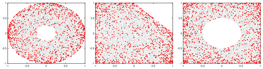
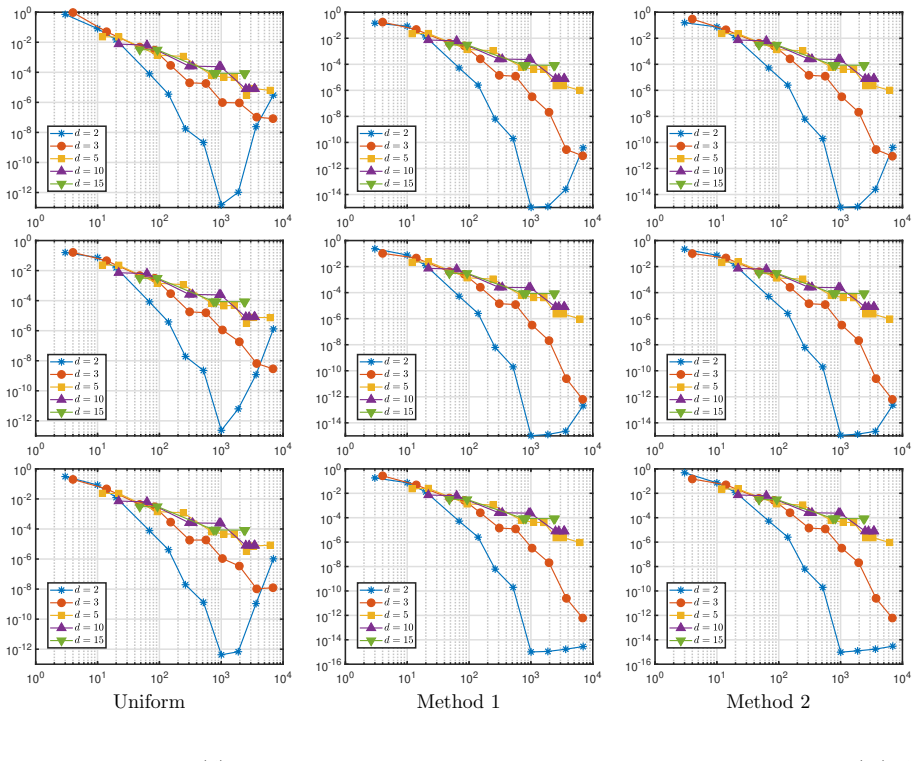
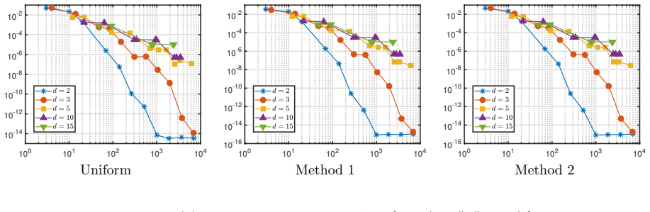
- [Abstract, Theorem 2.1, Section 3.6] The title, abstract, and Theorem 2.1 present the result as a provable accuracy guarantee on general domains, but the L2(Ω,ρ) error bound requires K to satisfy the condition involving N(P,ρ) in Theorem 2.1, and an explicit bound on N(P,ρ) is proven only for λ-rectangle domains with lower-set polynomial spaces and uniform ρ (Proposition 3.6). Remark 3.7 explicitly states that for balls and simplices, and more generally for irregular domains, the Nikolskii constant is unknown, and Section 6 repeats this limitation. The numerical examples in Fig. 1 include a simplex (Ω2) and an exterior-of-ball domain (Ω3) that are not covered by Proposition 3.6, and Fig. 4 shows that for K = 20000 the off-grid error can be orders of magnitude larger than the on-grid error. The abstract and Theorem 2.1 should be qualified to state that the whole-domain accuracy guarantee is conditional on a known/effective bound for N(P,ρ), or the authors should add explicit Nikolskii bounds for at least some non-λ-rectangle domains.
- [Theorems 2.1 and 2.2, proof of Theorem 2.1] In the statement of Theorem 2.1 and in its proof, the norm |||g|||_{Z,π} is defined as max_{i=1,...,K} |g(z_i)|√(Kπ_i). However, from (3.13) and (3.14), w(z_i) = 1/(Kπ_i), so √(w(z_i))|g(z_i)| = |g(z_i)|/√(Kπ_i), not |g(z_i)|√(Kπ_i). Thus the displayed identity in the proof of Theorem 2.1 and the definition in Theorem 2.1(iii) appear to be the reciprocal of the correct weighted sup-norm. If the formula as printed is intended, the bound in Theorem 2.1(iii) does not follow from Theorem 3.1; if it is a typographical omission of a division sign, it must be corrected. The same issue affects the definition of |||g|||_{Z,π,t} in Theorem 2.2.
minor comments (4)
- [Section 3.1, Eqs. (3.6) and (3.7)] The definitions of C and D use the condition p|supp(τ) ≠ 0 and p|supp(ρ) ≠ 0 to exclude a zero denominator, but the denominator is ‖p‖_{Υ,w} and ‖p‖_{L2(Ω,τ)}, respectively, and a function can be nonzero on the support while vanishing on the sample points or the grid. The intended condition is that the denominator be nonzero, or equivalently that the relevant semi-norm be a norm on P.
- [Throughout] There are several typographical errors, including 'simplicies' in Remark 3.7 (should be 'simplices') and 'with resect to' in the proof of Theorem 4.1 (should be 'with respect to'). A careful copyedit is recommended.
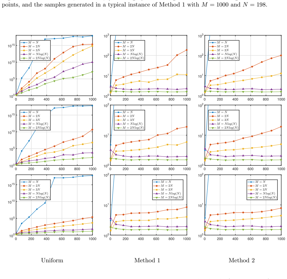
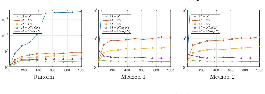
- [Section 5, Fig. 3] The text describing Fig. 3 refers to different scalings of M with N, but it is not clear from the caption or the text which curves correspond to M = cN versus M = cN log N. Please identify the scalings in the caption or legend.
- [Section 2.1] The sentence stating that ∑|φ_i(y)|^2 is the reciprocal of the Christoffel function is correct but would be clearer if it noted that the Christoffel function itself is typically defined as the reciprocal of this sum.
Circularity Check
No significant circularity: the sampling measure is constructed from the approximation space alone, the main probability bounds are proven from concentration inequalities, and the imported Nikolskii estimates are independent external results.
full rationale
The paper's derivation chain is not circular. The discrete sampling measure is defined solely from the approximation space P and the randomly generated K-point grid: after the QR decomposition B = QR, the weights are pi_i = (1/N) sum_j |q_ij|^2, which is the Christoffel function of P with respect to the discrete orthogonality measure tau. No target-function values are used to construct the measure, and no fitted parameter is renamed as a prediction. The M = O(N log N) sample-complexity bound is obtained through the Matrix Chernoff inequality in Theorem 4.1 and the exact identity N(P,tau,w) = sqrt(N) for the Christoffel choice of w, so the conditioning and grid-error statements are derived, not assumed. The only external ingredients are the Nikolskii bounds used to control the grid-size constant D: Proposition 3.4 cites [4, Thm. 6.2] and Proposition 3.6 cites [4, Thm. 6.6]. These are self-citations by the first author, but they are parameter-free mathematical results with explicitly stated assumptions (lambda-rectangle property, lower-set polynomial spaces, uniform measure) that do not include the paper's target error bound, and they were developed for a different framework; hence they constitute independent support rather than a circular premise. The acknowledged limitation that no K guarantee is proven for balls, simplices, or other irregular domains (Remark 3.7 and Section 6) is an honest scope restriction, not a circularity: it means the general-domain claim is conditional on knowing the Nikolskii constant, but it does not make any theorem reduce to its own input. The numerical observation in Fig. 4 that off-grid errors can be much larger than on-grid errors is likewise an empirical limitation consistent with an uncontrolled D, not evidence that the method's predictions are manufactured from its assumptions.
Assumptions & free parameters
assumptions (5)
- standard math Matrix Chernoff inequality holds and is applicable to the sum of independent self-adjoint matrices.
- standard math The reduced QR decomposition of the K by N matrix B provides an orthonormal basis for P with respect to the discrete grid measure.
- domain assumption For a lambda-rectangle domain and lower-set polynomial spaces, the Nikolskii constant satisfies (N(P,rho))^2 <= N^2/lambda.
- domain assumption The error measure rho can be sampled efficiently to generate the fine grid Z.
- domain assumption For every grid point there exists a function in P that does not vanish there.
Cite this review
Pith. "Pith review of Near-optimal sampling strategies for multivariate function approximation on general domains." pith.science (2026). https://pith.science/paper/2A44LDZS
@misc{pith2026190801249,
  author       = {Pith},
  title        = {Pith review of: Near-optimal sampling strategies for multivariate function approximation on general domains},
  year         = {2026},
  howpublished = {\url{https://pith.science/paper/2A44LDZS}},
  note         = {Machine review of arXiv:1908.01249}
}
abstract
In this paper, we address the problem of approximating a multivariate function defined on a general domain in $d$ dimensions from sample points. We consider weighted least-squares approximation in an arbitrary finite-dimensional space $P$ from independent random samples taken according to a suitable measure. In general, least-squares approximations can be inaccurate and ill-conditioned when the number of sample points $M$ is close to $N = \dim(P)$. To counteract this, we introduce a novel method for sampling in general domains which leads to provably accurate and well-conditioned approximations. The resulting sampling measure is discrete, and therefore straightforward to sample from. Our main result shows near-optimal sample complexity for this procedure; specifically, $M = \mathcal{O}(N \log(N))$ samples suffice for a well-conditioned and accurate approximation. Numerical experiments on polynomial approximation in general domains confirm the benefits of this method over standard sampling.
Figures

Figures from the paper (3 more)
Reference graph
Works this paper leans on
-
[1]
B. Adcock. Infinite-dimensional compressed sensing and function interpolation. Found. Comput. Math., 18(3):661–701, 2018
work page 2018
- [2]
- [3]
-
[4]
B. Adcock and D. Huybrechs. Approximating smooth, multivariate functions on irregular domains. arXiv:1802.00602, 2018
arXiv 2018
-
[5]
Frames and numerical approximation II: generalized sampling
B. Adcock and D. Huybrechs. Frames and numerical approximation II: generalized sampling. arXiv:1802.01950, 2018
work page Pith review arXiv 2018
-
[6]
B. Adcock and D. Huybrechs. Frames and numerical approximation. SIAM Rev., 61(3):443–473, 2019
work page 2019
- [7]
- [8]
Show all 27 references
-
[9]
Chkifa, N
A. Chkifa, N. Dexter, H. Tran, and C. G. Webster. Polynomial approximation via compressed sensing of high-dimensional functions on lower sets. Math. Comp., 2017
2017
-
[10]
Cohen, M
A. Cohen, M. A. Davenport, and D. Leviatan. On the stability and accuracy of least squares approxi- mations. Found. Comput. Math., 13:819–834, 2013
2013
-
[11]
Cohen and G
A. Cohen and G. Migliorati. Optimal weighted least-squares methods. SMAI Journal of Computational Mathematics, 3:181–203, 2017
2017
-
[12]
F. Dai, D. Gorbachev, and S. Tikhonov. Estimates of the asymptotic Nikolskii constants for spherical polynomials. arXiv:1907.03832, 2019
1907 arXiv
-
[13]
Doostan and H
A. Doostan and H. Owhadi. A non-adapted sparse approximation of PDEs with stochastic inputs. J. Comput. Phys., 230(8):3015–3034, 2011
2011
-
[14]
Hampton and A
J. Hampton and A. Doostan. Compressive sampling of polynomial chaos expansions: Convergence analysis and sampling strategies. J. Comput. Phys. , 280:363–386, 2015
2015
-
[15]
A. Kro´ o. Christoffel functions on convex and starlike domains inRd. J. Math. Anal. Appl., 421:718–729, 2015
2015
-
[16]
C. L. Lawson and R. J. Hanson. Solving Least Squares Problems, volume 15. SIAM, 1995
1995
-
[17]
Migliorati
G. Migliorati. Polynomial approximation by means of the random discrete L2 projection and application to inverse problems for PDEs with stochastic data . PhD thesis, Politecnico di Milano, 2013
2013
-
[18]
Migliorati
G. Migliorati. Multivariate Markov-type and Nikolskii-type inequalities for polynomials associated with downward closed multi-index sets. J. Approx. Theory, 189:137–159, 2015
2015
-
[19]
Migliorati
G. Migliorati. Adaptive approximation by optimal weighted least squares methods. arXiv:1807.00402, 2018
2018 arXiv
-
[20]
Migliorati
G. Migliorati. Multivariate approximation of functions on irregular domains by weighted least-squares methods. arXiv:1907.12304, 2019
1907 arXiv
-
[21]
Migliorati, F
G. Migliorati, F. Nobile, E. von Schwerin, and R. Tempone. Analysis of the discrete L2 projection on polynomial spaces with random evaluations. Found. Comput. Math., 14:419–456, 2014
2014
-
[22]
Narayan, J
A. Narayan, J. D. Jakeman, and T. Zhou. A Christoffel function weighted least squares algorithm for collocation approximations. arXiv:1412.4305, 2014
2014 arXiv
-
[23]
Narayan and T
A. Narayan and T. Zhou. Stochastic collocation on unstructured multivariate meshes. Commun. Comput. Phys., 18(1):1–36, 2015
2015
-
[24]
P. Nevai. G´ eza Freud, orthogonal polynomials and Christoffel functions. A case study. J. Approx. Theory, 48(1):3–167, 1986
1986
-
[25]
Prymak and O
A. Prymak and O. Usoltseva. Christoffel function on planar domains with piecewise smooth boundary. Acta Math. Hungar. , 158(1):216–234, 2019
2019
-
[26]
J. A. Tropp. User friendly tail bounds for sums of random matrices. Found. Comput. Math., 12:389–434, 2012
2012
-
[27]
Y. Xu. Orthogonal polynomials and cubature formulae on spheres and on balls. SIAM J. Math. Anal. , 29(3):778–793, 1998. 24
1998
Reviewed August 14, 2026 · model on record in the stance chip above.
Discussion (0). Continue with ORCID to comment.