REVIEW 4 major objections 5 minor 55 references
The Double Emulator
T0 review · 4 major / 5 minor · reviewed 2026-08-12 · deepseek-v4-flash
Pith's one-line read A mixture of a point mass at the known minimum and a lognormal GPE predicts better than the plain GPE for simulators that reach their minimum over a substantial region, and most so when the landing is hard.
desk verdict An appealing method with a correctable but load-bearing error: the CRPS comparisons rely on an invalid CDF that needs fixing before the empirical claims can be trusted. read the letter →
The pith
A machine-rendered reading of the paper's core claim, the machinery that carries it, and where it could break.
The reading
What carries the argument
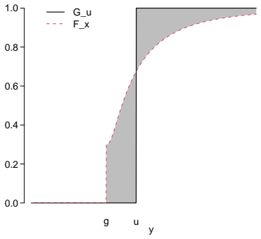
The central object is the double emulator distribution of Definition 3.1, $F(y;x)=0$ for $y<g$, $F(g;x)=1-p(x)$, and $F(y;x)=1-p(x)+p(x)L(y-g+\gamma;m(x),v(x))$ for $y>g$, where $L$ is the lognormal distribution. The mixture's mean and variance come from the law of total expectation and total variance: $\mathbb{E}S(x)=(1-p(x))g+p(x)M(x)$ and $\mathrm{Var}\,S(x)=p(x)(1-p(x))(g-M(x))^2+p(x)V(x)$. Lemma 4.1 gives the CRPS in closed form, so the mixture can be scored exactly without numerical integration. The point mass carries the load: it encodes the known minimum with zero uncertainty, while the classifier supplies $p(x)$ and therefore locates the unknown grounding line.
What would settle it
Fit both models to the same training design on a simulator with a known hard landing and a moderate grounded region, then compare CRPS restricted to a thin band of test inputs around the grounding line; the paper's claim predicts the double emulator dominates there and that the gap grows with the derivative jump, so a flat or reversed comparison in that band would refute the core claim.
Extended reading notes
Core claim
The paper's central claim is that the double emulator—defined in Definition 3.1 as a mixture of a point mass at the known minimum $g$ and a lognormal Gaussian process (GPE) tail, with the mixing weight $p(x)=P(S(x)>g)$ estimated by a probabilistic classifier—is a better emulator than a plain GPE for simulators that ground. The paper attributes the plain GPE's failure to a tension in its Gram matrix: training pairs that straddle the grounding line push the estimated lengthscale toward wiggliness, while pairs on one side push it toward smoothness, so no stationary correlation function fits both. The double emulator avoids this by returning the known minimum with zero uncertainty wherever the classifier says the simulator has grounded, and fitting a lognormal GPE only to the non-grounded tail. Empirically, on the curved and Banana synthetic families and on the uranium oxidation simulator, this yields lower CRPS and competitive RMSE for moderate grounded volumes, with the largest gains for hard landings; for very large grounded volumes the plain GPE can win back, and classifier quality matters more for CRPS than for RMSE.
Load-bearing premise
The method depends on the classifier's probability estimates being trustworthy near the boundary where the simulator reaches its minimum, since those probabilities decide how much weight the point mass at the known minimum receives.
Editorial extensions
If this is right
- On simulators with a grounded region of moderate volume, the double emulator should give better probabilistic predictions than the plain GPE, as measured by CRPS, and comparable or better RMSE.
- The improvement over the GPE should grow as the change in the simulator's derivative across the grounding line grows, so the method is most valuable for hard landings.
- When the grounded region occupies a very large share of the input space, the double emulator can lose to the GPE, so practitioners should use the plain GPE or stabilize the GPE component in that regime.
- A better classifier (closer to an omniscient one) almost always improves CRPS, whereas its effect on RMSE is less clear, indicating that classifier quality chiefly buys calibration.
- The closed-form CRPS for the mixture means the double emulator can be evaluated and compared without numerical integration over the atom at the minimum.
Reading between the lines
- The paper frames the point mass as specific to a known minimum, but the same mixture construction would apply to any known structural feature of simulator output, such as a saturation level or a failure threshold, provided the classifier can identify where that feature holds.
- The failure at large grounded volumes is blamed on the GPE component starving for non-grounded data; this suggests a testable fix of allocating training runs by a design that targets the grounding line, which the paper mentions as ongoing work.
- Because the advantage tracks the derivative jump, one could estimate that jump from the training data and use it as a trigger for switching between GPE and double emulator in an automated emulation pipeline.
- The paper restricts the tail to a lognormal GPE; combining the point-mass mixture with nonstationary or warped kernels inside the tail would likely extend the gains to simulators where the non-grounded region itself is nonstationary.
Editorial analysis
A structured set of objections, weighed in public.
Referee Report
Summary. This paper proposes the 'double emulator', a predictive model for deterministic simulators that attain a known minimum g on a substantial region of the input space ('grounding'). The predictive distribution is a mixture: with probability 1-p(x) the output is exactly g, and with probability p(x) it follows a shifted, log-transformed Gaussian process, where p(x) is estimated by a probabilistic classifier (random forest or SVM) trained on the indicator of whether each training run equals g; a perfect-classifier oracle is included as a benchmark. The authors derive closed-form expressions for the predictive mean, variance, and CRPS (Definition 3.1; Lemmas 3.2 and 4.1), then compare the double emulator with a conventional stationary GPE on two synthetic families (Dette-Pepelyshev and Rosenbrock) with controlled grounded volume and landing hardness, and on a uranium oxidation simulator. The reported conclusions are that the double emulator regularly outperforms the GPE in CRPS for moderate grounded volumes and hard landings, that the advantage grows as the landing becomes harder, and that the GPE is better when the grounded volume is very large.
Significance. If the claims held up, the paper would add a simple and useful tool for a common failure mode of stationary GPEs, and several strengths are real: the empirical protocol is honest (held-out test sets, ten Monte Carlo repetitions per setting, a perfect-classifier oracle that isolates the classifier effect, and explicit reporting of the GV=0.8 and imbalanced-class regimes where the method fails); the supplementary material promises R code and data; and the algebra leading to Lemmas 3.2 and 4.1 is checkable. However, the central object, the distribution function in Definition 3.1, is not a valid CDF, and the mean, variance, and CRPS formulae derived from it are not the moments and scores of any well-defined predictive distribution. Since the headline claims (Introduction items 1 and 3) rest on the CRPS formula, the reported numerical support for the method is not currently valid. The defect is repairable within the paper's scope, namely by respecifying the mixture with a truncated lognormal component, but the experiments must be re-run before the claims can be assessed.
major comments (4)
- [Definition 3.1 (Eq. 7)] Eq. (7) does not define a valid cumulative distribution function, so there is no random variable with this distribution. For y>g the definition gives F(y)=1-p(x)+p(x)L(y-g+gamma), while F(g)=1-p(x); since gamma>0 and the lognormal CDF satisfies L(gamma)>0, the right limit at g is F(g+)=1-p+pL(gamma)>F(g), violating right-continuity. Equivalently, for every epsilon>0 the interval (g,g+epsilon] receives probability F(g+epsilon)-F(g)=pL(gamma+epsilon)>=pL(gamma)>0, while the nested intervals (g,g+epsilon] decrease to the empty set as epsilon decreases, violating countable additivity. The root cause is that the shifted lognormal component Y-g+gamma~Lognormal(m,v) has positive probability on (g-gamma,g), so the atom of mass 1-p at g and the zero CDF below g cannot coexist with it; a consistent untruncated specification would need F(y)=pL(y-g+gamma) for g-gamma<y<g and F(g)=1-p+pL(gamma), while a consistent truncated specification would use (L(y-g+gamma)-L(gamma))/(1-L(gamma)) above g. Near the grounding line the GPE mean m(x) is close to ln(gamma), so L(gamma) is approximately 1/2 and the anomalous mass is O(p), not a negligible technicality. The model must be respecified and all subsequent formulae re-derived.
- [Lemma 3.2 (Eqs. 9-11)] The mean and variance in (9)-(11) use the untruncated lognormal moments but are presented as the moments of the mixture (7). Under any internally consistent version of the intended model, in which non-grounded means S(x)>g, the conditional distribution of Z=Y-g+gamma must be truncated to Z>gamma, and E[Z|Z>gamma]=e^{m+v/2} Phi((m+v-ln(gamma))/sqrt(v))/Phi((m-ln(gamma))/sqrt(v)), which strictly exceeds the untruncated e^{m+v/2}; setting m=ln(gamma) gives approximately 2e^{m+v/2}Phi(sqrt(v)). Consequently M(x) in (9) is too small near the grounding line, and the double-emulator mean (10) and variance (11) are the moments of a misspecified model. Because the RMSE comparisons in Supplement D and the credible-interval plots in Figures 2, 8, and 9 are built on (10)-(11), these results inherit the misspecification; the bias is largest exactly where the method claims its main advantage.
- [Lemma 4.1 (Eq. 13) and Supplement B.2 (Eqs. 22-24)] Eq. (13) is not the CRPS of a well-defined predictive distribution, because the CRPS is defined for distribution functions and (7) is not one. The algebra in the proof of Lemma 4.1 correctly evaluates the integral of squared differences for the function F in (7), but that integral is a functional of an invalid CDF, so the values plotted in Figures 4, 6, 10, and 12 (and the 1D CRPS panels in Figures 8-9) do not measure the CRPS of the double-emulator model. For a properly truncated mixture the integrand would involve (L(z)-L(gamma))/(1-L(gamma)) rather than L(z); with m(x) close to ln(gamma) near the grounding line, L(gamma) is approximately 1/2, so the discrepancy is O(p) in the very region where the method claims its main benefit. In addition, Eq. (24) in Supplement B.2 is itself incorrect: for gamma>0, CRPS(L,gamma) equals the integral from 0 to gamma of L(z)^2 dz plus the integral from gamma to infinity of (L(z)-1)^2 dz, so the asserted equality between the latter integral and CRPS(L,gamma) omits the positive term integrable over (0,gamma). Since the paper's central claims (Introduction items 1 and 3) are supported by these CRPS comparisons, they are unsupported as stated until the formula is re-derived and the experiments re-run.
- [Section 4 (empirical scope)] The experimental comparison includes only the vanilla stationary GPE as a baseline, although the Introduction motivates the work with the failure of stationary emulation and cites deep GPs, non-stationary kernels, input warping, kernel mixtures, and treed GPs as existing alternatives. Adding at least one such baseline, for example a treed GP (Gramacy and Lee, 2008) or a warped GP (Snelson et al., 2003), both of which are straightforward to fit, would substantially strengthen the positioning of the method; as it stands the experiments support only the narrow claim that the double emulator beats a stationary GPE using the same kernel, not the broader positioning against the non-stationary emulation toolbox that the paper cites.
minor comments (5)
- [Section 3.1] The constant gamma, described as a small positive constant improving the stability of the log-scale emulation, is never assigned a value or a selection rule, although the behavior of the model near the grounding line depends on it; please state the value used in the experiments and report sensitivity to it.
- [Section 4.1] The paper excludes cases where the out-of-the-box SVM throws error messages on highly imbalanced classes; please report how many such cases were excluded in each Monte Carlo setting, since the exclusions are concentrated in the GV=0.8 regime that the paper singles out for discussion.
- [Supplement D] The text of Supplement D promises the RMSE results for the Banana simulator, but Figure 12 is captioned as CRPS for the simulator in (15), duplicating Figure 4, while the promised Banana RMSE figure appears to be missing; the caption-to-text mapping for Figures 10-12 should be corrected.
- [Figure 3] The caption of Figure 3 spells the first function name as Dettel and Pepelyshev; it should be Dette and Pepelyshev.
- [Figures 4 and 6] The CRPS and RMSE axes in Figures 4 and 6 are on a logarithmic scale, but the axis labels and captions do not say so (for Figure 6 the log scale is mentioned only in the text); please label the axes accordingly.
Circularity Check
No significant circularity: the double emulator is a derived probabilistic model with parameters fitted to training data and evaluated on held-out test sets.
full rationale
The paper's derivation chain is self-contained and does not reduce any prediction to its own inputs. Definition 3.1 specifies a probabilistic mixture model for the simulator output; the classifier probability p(x) and the lognormal GPE parameters m(x) and v(x) are estimated from training data, and the RMSE and CRPS comparisons in Section 4 use held-out test sets that were not used for fitting. The CRPS expression in Lemma 4.1 is derived analytically from the model's distribution function rather than tuned to match the observed scores, and kernel hyperparameters are estimated using RobustGaSP before evaluation with the same settings for both the GPE and the double emulator. The central claim that the double emulator outperforms the GPE on moderate grounded volumes is an empirical result obtained by comparing the two models on the same test data, not an algebraic consequence of a fitted parameter relabeled as a prediction. There is a mathematical issue with Definition 3.1 regarding right-continuity at the grounding value g, and the resulting CRPS formula inherits that issue, but that is a correctness concern rather than circularity. Self-citations are present but only provide background or standard methodology, and no load-bearing argument depends on an unverified self-cited theorem. Overall, the evaluation is statistically honest and externally grounded in simulator runs. Score 0.
Assumptions & free parameters
free parameters (4)
- gamma (log-shift constant) =
small positive constant, value not stated
- GPE kernel hyperparameters lambda_j =
estimated per dataset via RobustGaSP defaults
- classifier default hyperparameters =
defaults in kernlab and randomForest packages
- grounding threshold g =
square root of machine precision for the oxidation simulator
assumptions (3)
- domain assumption Simulator output is deterministic, bounded below by a known g, and exactly equal to g throughout the grounded region.
- domain assumption Non-grounded outputs, after the transform Y-g+gamma, follow a Lognormal distribution whose log-mean and log-variance are given by a stationary Gaussian process.
- domain assumption A probabilistic classifier with default settings provides a usable estimate of P(S(x)>g), including near the grounding line.
Cite this review
Pith. "Pith review of The Double Emulator." pith.science (2026). https://pith.science/paper/2BBT3E6W
@misc{pith2026241114005,
  author       = {Pith},
  title        = {Pith review of: The Double Emulator},
  year         = {2026},
  howpublished = {\url{https://pith.science/paper/2BBT3E6W}},
  note         = {Machine review of arXiv:2411.14005}
}
read the original abstract
Computer models (simulators) are vital tools for investigating physical processes. Despite their utility, the prohibitive run-time of simulators hinders their direct application for uncertainty quantification. Gaussian process emulators (GPEs) have been used extensively to circumvent the cost of the simulator and are known to perform well on simulators with smooth, stationary output. In reality, many simulators violate these assumptions. Motivated by a finite element simulator which models early stage corrosion of uranium in water vapor, we propose an adaption of the GPE, called the double emulator, specifically for simulators which 'ground' in a considerable volume of their input space. Grounding is the process by which a simulator attains its minimum and can result in violation of the stationarity and smoothness assumptions used in the conventional GPE. We perform numerical experiments comparing the performance of the GPE and double emulator on both the corrosion simulator and synthetic examples.
Figures


Figures from the paper (9 more)




Reference graph
Works this paper leans on
-
[1]
Baran, S. and Lerch, S. (2015). Log-normal distribution based Ensemble Model Output Statistics models for probabilistic wind-speed forecasting. Quarterly Journal of the Royal Meteorological Society\/ , 141, 691, 2289--2299
work page 2015
-
[2]
Bayarri, M. J., Berger, J. O., Calder, E. S., Dalbey, K., Lunagomez, S., Patra, A. K., Pitman, E. B., Spiller, E. T., and Wolpert, R. L. (2009). Using statistical and computer models to quantify volcanic hazards. Technometrics\/ , 51, 4, 402--413
work page 2009
-
[3]
Breiman, L. (2001). Random forests. Machine learning\/ , 45, 5--32
work page 2001
-
[4]
Casella, G. and Berger, R. (2002). Statistical Inference\/ . Duxbury advanced series in statistics and decision sciences. Thomson Learning
work page 2002
-
[5]
Cole, D. A., Gramacy, R. B., Warner, J. E., Bomarito, G. F., Leser, P. E., and Leser, W. P. (2023). Entropy-based adaptive design for contour finding and estimating reliability. Journal of Quality Technology\/ , 55, 1, 43–60
work page 2023
-
[6]
Cortes, C. and Vapnik, V. (1995). Support-vector networks. Machine Learning\/ , 20, 3, 273–297
work page 1995
-
[7]
Currin, C., Mitchell, T., Morris, M., and Ylvisaker, D. (1991). Bayesian prediction of deterministic functions, with applications to the design and analysis of computer experiments. Journal of the American Statistical Association\/ , 86, 416, 953--963
work page 1991
-
[8]
Damianou, A. and Lawrence, N. D. (2013). Deep Gaussian Processes. In Proceedings of the Sixteenth International Conference on Artificial Intelligence and Statistics\/ , 207–215. PMLR
work page 2013
Show all 55 references
-
[9]
Dean, A., Morris, M., Stufken, J., and Bingham, D. (2015). Handbook of Design and Analysis of Experiments\/ . Chapman & Hall/CRC Handbooks of Modern Statistical Methods. CRC Press
2015
-
[10]
and Pepelyshev, A
Dette, H. and Pepelyshev, A. (2010). Generalized Latin Hypercube Design for Computer Experiments. Technometrics\/ , 52, 421–429
2010
-
[11]
M., Girolami, M
Dunlop, M. M., Girolami, M. A., Stuart, A. M., and Teckentrup, A. L. (2018). How deep are deep Gaussian processes? Journal of Machine Learning Research\/ , 19, 54, 1--46
2018
-
[12]
and Raftery, A
Gneiting, T. and Raftery, A. E. (2007). Strictly Proper Scoring Rules, Prediction, and Estimation. Journal of the American Statistical Association\/ , 102, 477, 359–378
2007
-
[13]
and Strange, R
Godfrey, H. and Strange, R. (2020). Knowledge S tatus on U ranium H ydride
2020
-
[14]
and Rougier, J
Goldstein, M. and Rougier, J. (2004). Probabilistic Formulations for Transferring Inferences from Mathematical Models to Physical Systems. SIAM J. Sci. Comput.\/
2004
-
[15]
Gramacy, R. B. (2020). Surrogates: G aussian Process Modeling, Design and Optimization for the Applied Sciences\/ . Boca Raton, Florida: Chapman Hall/CRC
2020
-
[16]
Gramacy, R. B. and Apley, D. W. (2015). Local Gaussian process approximation for large computer experiments. Journal of Computational and Graphical Statistics\/ , 24, 2, 561--578
2015
-
[17]
Gramacy, R. B. and Lee, H. K. H. (2008). Bayesian Treed Gaussian Process Models with an Application to Computer Modeling. Journal of the American Statistical Association\/ , 103, 483, 1119–1130
2008
-
[18]
Gu, M., Palomo, J., and Berger, J. O. (2022). R obust G a SP : R obust G aussian S tochastic P rocess E mulation. R package
2022
-
[19]
Gu, M., Wang, X., and Berger, J. O. (2018). Robust Gaussian Stochastic Process Emulation. The Annals of Statistics\/ , 46, 6A, 3038–3066
2018
-
[20]
Hastie, T., Tibshirani, R., and Friedman, J. (2009). The Elements of Statistical Learning\/ . Springer Series in Statistics. New York, NY: Springer
2009
-
[21]
Higdon, D. (1998). A process-convolution approach to modelling temperatures in the North Atlantic Ocean. Environmental and Ecological Statistics\/ , 5, 2, 173–190
1998
-
[22]
Higdon, D., Gattiker, J., Williams, B., and Rightley, M. (2008). Computer M odel C alibration U sing H igh- D imensional O utput. Journal of the American Statistical Association\/ , 103, 482, 570--583
2008
-
[23]
C., Cafeo, J
Higdon, D., Kennedy, M., Cavendish, J. C., Cafeo, J. A., and Ryne, R. D. (2004). Combining Field Data and Computer Simulations for Calibration and Prediction. SIAM Journal on Scientific Computing\/ , 26, 2, 448–466
2004
-
[24]
and Welch, W
Isberg, S. and Welch, W. J. (2022). Adaptive Design and Analysis Via Partitioning Trees for Emulation of a Complex Computer Code. Journal of Computational and Graphical Statistics\/ , 31, 4, 1280–1291
2022
-
[25]
Karatzoglou, A., Smola, A., Hornik, K., and Zeileis, A. (2004). kernlab -- An S4 Package for Kernel Methods in R . Journal of Statistical Software\/ , 11, 9, 1--20
2004
-
[26]
Kennedy, M. C. and O’Hagan, A. (2001). Bayesian calibration of computer models. Journal of the Royal Statistical Society: Series B (Statistical Methodology)\/ , 63, 3, 425–464
2001
-
[27]
and Sandrock, C
Kok, S. and Sandrock, C. (2009). Locating and characterizing the stationary points of the extended Rosenbrock function. Evolutionary Computation\/ , 17, 3, 437–453
2009
-
[28]
and Wiener, M
Liaw, A. and Wiener, M. (2002). Classification and Regression by randomForest. R News\/ , 2, 3, 18--22
2002
-
[29]
Marques, A., Lam, R., and Willcox, K. (2018). Contour location via entropy reduction leveraging multiple information sources. In Advances in Neural Information Processing Systems\/ , vol. 31. Curran Associates, Inc
2018
-
[30]
D., Beckman, R
McKay, M. D., Beckman, R. J., and Conover, W. J. (1979). A Comparison of Three Methods for Selecting Values of Input Variables in the Analysis of Output from a Computer Code. Technometrics\/ , 21, 2, 239–245
1979
-
[31]
Mockus, J., Tiesis, V., and Zilinskas, A. (1978). The application of Bayesian methods for seeking the extremum\/ , vol. 2, 117--129
1978
-
[32]
Natchiar, M. (2021). Mathematical Modelling of Diffusion-Driven Oxidation in Metals. Ph.D. thesis, University of Manchester
2021
-
[33]
E., Monks, P
Natchiar, M., Hewitt, R. E., Monks, P. D. D., and Morrall, P. (2020). Asymptotics of Coupled Reaction-Diffusion Fronts With Multiple Static and Diffusing Reactants: Uranium Oxidation in Water Vapor. SIAM Journal on Applied Mathematics\/ , 80, 5, 2249–2270
2020
-
[34]
Paciorek, C. (2003). Nonstationary Gaussian Processes for Regression and Spatial Modelling. Ph.D. thesis, Carnegie Mellon
2003
-
[35]
and Schervish, M
Paciorek, C. and Schervish, M. (2003). Nonstationary Covariance Functions for Gaussian Process Regression. In Advances in Neural Information Processing Systems\/ , vol. 16. MIT Press
2003
-
[36]
Picheny, V., Wagner, T., and Ginsbourger, D. (2013). A benchmark of kriging-based infill criteria for noisy optimization. Structural and multidisciplinary optimization\/ , 48, 607--626
2013
-
[37]
Platt, J. et al. (1999). Probabilistic outputs for support vector machines and comparisons to regularized likelihood methods. Advances in large margin classifiers\/ , 10, 3, 61--74
1999
-
[38]
R: A Language and Environment for Statistical Computing\/
R Core Team (2024). R: A Language and Environment for Statistical Computing\/ . R Foundation for Statistical Computing, Vienna, Austria
2024
-
[39]
Ranjan, P., Bingham, D., and Michailidis, G. (2008). Sequential experiment design for contour estimation from complex computer codes. Technometrics\/ , 50, 4, 527--541
2008
-
[40]
Rasmussen, C. E. and Williams, C. K. I. (2005). Gaussian Processes For Machine Learning\/ . MIT
2005
-
[41]
Rosenbrock, H. H. (1960). An Automatic Method for Finding the Greatest or Least Value of a Function . The Computer Journal\/ , 3, 3, 175--184
1960
-
[42]
Rougier, J. C. (2008). Efficient Emulators for Multivariate Deterministic Functions. Journal of Computational and Graphical Statistics\/ , 17, 4, 827–843
2008
-
[43]
C., Guillas, S., Maute, A., and Richmond, A
Rougier, J. C., Guillas, S., Maute, A., and Richmond, A. D. (2009). Expert Knowledge and Multivariate Emulation: The Thermosphere–Ionosphere Electrodynamics General Circulation Model (TIE-GCM). Technometrics\/ , 51, 4, 414–424
2009
-
[44]
and Notz, W
Roy, S. and Notz, W. I. (2014). Estimating percentiles in computer experiments: a comparison of sequential-adaptive designs and fixed designs. Journal of Statistical Theory and Practice\/ , 8, 12--29
2014
-
[45]
J., Mitchell, T
Sacks, J., Welch, W. J., Mitchell, T. J., and Wynn, H. P. (1989). Design and Analysis of Computer Experiments. Statistical Science\/ , 4, 4, 409–423
1989
-
[46]
Sampson, P. D. and Guttorp, P. (1992). Nonparametric Estimation of Nonstationary Spatial Covariance Structure. Journal of the American Statistical Association\/ , 87, 417, 108–119
1992
-
[47]
J., Williams, B
Santner, T. J., Williams, B. J., and Notz, W. I. (2018). The Design and Analysis of Computer Experiments\/ . Springer Series in Statistics. Springer
2018
-
[48]
Sauer, A., Cooper, A., and Gramacy, R. B. (2023). Vecchia-Approximated Deep Gaussian Processes for Computer Experiments. Journal of Computational and Graphical Statistics\/ , 32, 3, 824–837
2023
-
[49]
Schonlau, M. (1997). Computer experiments and global optimization. Ph.D. thesis, University of Waterloo
1997
-
[50]
J., and Jones, D
Schonlau, M., Welch, W. J., and Jones, D. R. (1998). Global versus local search in constrained optimization of computer models. Lecture notes-monograph series\/ , 11--25
1998
-
[51]
Snelson, E., Ghahramani, Z., and Rasmussen, C. (2003). Warped Gaussian Processes. In Advances in Neural Information Processing Systems\/ , eds. S. Thrun, L. Saul, and B. Sch\" o lkopf, vol. 16. MIT Press
2003
-
[52]
Stein, M. L. (1999). Interpolation of S patial D ata: S ome T heory for K riging\/ . Springer, New York, NY
1999
-
[53]
and Williamson, D
Volodina, V. and Williamson, D. (2020). Diagnostics-driven nonstationary emulators using kernel mixtures. SIAM/ASA Journal on Uncertainty Quantification\/ , 8, 1, 1--26
2020
-
[54]
, " * write output.state after.block = add.period write newline
ENTRY address author booktitle chapter edition editor howpublished institution journal key month note number organization pages publisher school series title type volume year label extra.label sort.label short.list INTEGERS output.state before.all mid.sentence after.sentence a...
-
[55]
write newline
" write newline "" before.all 'output.state := FUNCTION n.dashify 't := "" t empty not t #1 #1 substring "-" = t #1 #2 substring "--" = not "--" * t #2 global.max substring 't := t #1 #1 substring "-" = "-" * t #2 global.max substring 't := while if t #1 #1 substring * t #2 gl...
Reviewed August 12, 2026 · model on record in the stance chip above.
Discussion (0). Continue with ORCID to comment.