REVIEW 3 major objections 5 minor 3 references
Regularized joint mixture models
T0 review · 3 major / 5 minor · reviewed 2026-08-14 · deepseek-v4-flash
Pith's one-line read A joint mixture model couples sparse feature graphs with sparse regressions so that latent groups can be learned from either signal, with EM convergence proved under a penalty condition.
desk verdict Useful joint mixture framework with strong simulations; the convergence theorem's key penalty condition doesn't hold for the implemented FLasso/NJ penalties, so the theoretical guarantee is weaker than claimed. read the letter →
The pith
A machine-rendered reading of the paper's core claim, the machinery that carries it, and where it could break.
The reading
What carries the argument
The central object is the regularized joint mixture (RJM) model, defined by a latent group indicator $Z$, a multivariate normal distribution for $X\mid Z$ with group-specific mean and inverse covariance $\Omega_k$, and a normal linear regression $Y\mid X,Z$ with group-specific intercept, coefficient vector, and variance. The machinery carrying the argument is the block-wise EM (ECM) objective, which splits into $Q_X$ for the graphical model, $Q_Y$ for the regression, and $Q_Z$ for group proportions, together with the penalty lower-bound condition (36) used in Theorem 2 to prove compact level sets and hence convergence of the ECM sequence to stationary points of $L(\xi)$.
What would settle it
Evaluate condition (36) on a fitted solution: for the FLasso penalty, $\mathrm{pen}(\xi)=-\lambda\|\phi\|_1-\zeta\|\Omega\|_1$ can be negative while the right-hand side is positive, so the inequality fails; alternatively, run the ECM with FLasso on a two-group simulation and track the penalized objective to see whether it cycles instead of settling at one value.
Extended reading notes
Core claim
The paper's central discovery is that the mixture model formed by coupling a Gaussian graphical model for the features and a normal linear regression for the response, with penalties specific to each latent group, breaks the equivalence between cluster-weighted models and a Gaussian mixture on the concatenated vector $(X,Y)$. That equivalence holds under maximum likelihood, but not under the regularized objective, and the breaking is what lets the regression and covariance signals each contribute to group allocation. The paper's Theorem 2 states that if the penalty is continuous, differentiable, gives unique block maximizations, and grows at least linearly in the norms and log-terms of all group parameters, then every limit point of the ECM sequence is a stationary point of the penalized observed log-likelihood. The theorem is stated as not applying directly to the random-penalty lasso variant, whose objective changes at each step, while the fixed-penalty lasso and normal-Jeffreys implementations are the intended beneficiaries of the guarantee.
Load-bearing premise
The proof requires the penalty to grow with the size of the parameters, but the penalties used in the implemented methods subtract rather than add parameter sizes; if that requirement is not met, the convergence guarantee does not apply to those methods.
Editorial extensions
If this is right
- Subgroup recovery can exploit regression-coefficient differences that are invisible to clustering on $X$ alone, and can exploit covariance differences that regression-only methods ignore.
- With both sources coupled, the model provides group-specific regression coefficients, conditional-independence graphs, and a group-specific prediction rule for a new feature vector.
- Regularization keeps per-group estimates well defined when the number of features is comparable to or larger than the sample size, a regime where unregularized cluster-weighted models fail.
- Ignoring latent groups and pooling the data can produce coefficient estimates with wrong signs, and the joint model avoids this by allowing groups to differ in both the feature and regression blocks.
- The number of groups can be selected by held-out predictive loss, connecting supervised and unsupervised model choice.
Reading between the lines
- The convergence theorem's sufficient condition (36) is not demonstrated for the negative $\ell^1$ penalties used in the FLasso and normal-Jeffreys implementations, so the behavior of those implemented methods rests on the empirical evidence rather than on the theorem.
- A natural testable extension would be to check condition (36) on actual parameter iterates, or to construct sparsity-inducing penalties that satisfy the lower bound while still acting like lasso or normal-Jeffreys shrinkage.
- The joint-modeling principle should transfer to generalized linear responses or longitudinal data, with the same expected benefit whenever group structure appears in both the feature distribution and the response mechanism.
- Because the model blocks data into distributionally non-identical groups, it could serve as a component of shift-robust learning, training and testing predictors across learned distributional regimes.
Signed reviews
Editorial analysis
A structured set of objections, weighed in public.
Referee Report
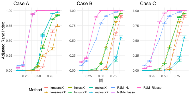
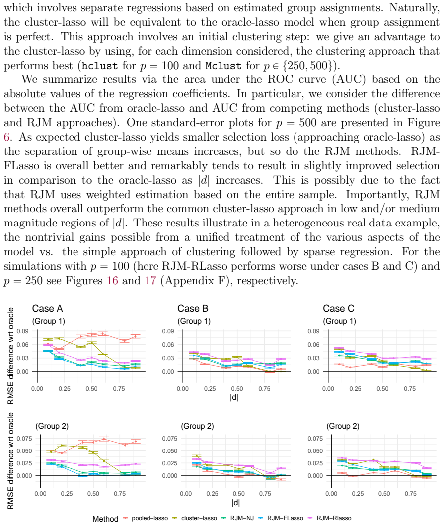
Summary. The paper proposes regularized joint mixture models (RJMs) for paired data (X, Y) with latent groups. Each mixture component contains a Gaussian graphical model for the feature distribution X and a linear regression for the conditional response Y|X, with group-specific parameters. Estimation is carried out by an expectation/conditional-maximization (ECM) algorithm that alternates between posterior membership weights and block updates for the means, inverse covariances, regression coefficients, and mixing proportions. Three regression penalties are implemented: FLasso (fixed lasso penalty via cross-validation), RLasso (random lasso penalty with a truncated Pareto prior), and NJ (normal-Jeffreys prior), together with a graphical lasso penalty on the inverse covariance matrices. The authors claim a theoretical convergence guarantee for the ECM algorithm and support the proposal with a small simulation study and semi-synthetic experiments based on TCGA data, comparing RJM variants against Gaussian mixtures, mixtures of experts, k-means, hierarchical clustering, cluster-then-lasso, and pooled lasso. An R package is referenced in the abstract.
Significance. If the claims were fully supported, the paper would offer a useful modular framework for joint clustering, sparse regression, and sparse graphical estimation in heterogeneous data, with a clear computational strategy and broad comparisons against established baselines. The strengths of the manuscript include the explicit model specification, the separation of the objective into X and Y blocks that makes the ECM updates simple, the use of standard well-tested solvers (glmnet, glassoFast), and simulation designs that probe realistic settings including p > n and real covariance structures. The central weakness is that the stated convergence theorem is not verified for the penalties actually implemented, so the headline theoretical claim is currently stronger than the proof supports. The empirical results remain of interest, but the theoretical claim needs to be either proved under conditions covering the implemented penalties or substantially qualified.
major comments (3)
- [Section 3.2.2, Eq. (36)/(42), and Section 2.2] Theorem 2 requires a positive constant delta such that pen(xi) >= delta times a sum including log(tau_k^{-1}), ||mu_k||, ||Omega_k||, log|Omega_k^{-1}|, rho_k, log(rho_k^{-1}), |chi_k|, and ||phi_k||. The penalties implemented in Section 2.2 do not satisfy this condition. The graphical lasso penalty is pen(Omega_k) = -zeta||Omega_k||_1 (Section 2.2.1), the FLasso penalty is effectively -lambda_k||phi_k||_1 in the coordinates used in Eq. (17) and Eq. (25), and the NJ penalty is sum_j log|beta_kj| (Eq. (12)), which is unbounded below as any coefficient approaches zero. None of these can dominate the unpenalized terms on the right-hand side of Eq. (36), and the FLasso/NJ penalties do not involve tau_k, mu_k, rho_k, or chi_k at all. The theorem therefore does not cover the methods used in the simulations; the paper explicitly excludes RLasso but does not exclude FLasso or NJ. The abstract's statement that convergence is 'established theoretically' is not supported for the implemented estimators and should be qualified.
- [Section 3.2.1, Theorem 1, Eq. (25), and FLasso in Section 2.2.2] The convergence theorem relies on the Meng-Rubin/Wu conditions, including uniqueness of every conditional maximization and a fixed objective function. The lasso update in Eq. (25) is an L1-penalized least squares problem; when p > n, which is one of the central settings in Section 5.2.2, the quadratic part is not strictly convex and the solution is not unique in general, so the uniqueness hypothesis is not automatically satisfied. In addition, the FLasso procedure re-estimates the penalty parameter lambda_k by cross-validation during the EM run, so the objective function changes at that iteration. The paper acknowledges that monotonicity may be disrupted but does not reconcile this with a theorem that assumes a fixed L(xi) and Q(xi|xi^{(t)}) throughout. These are additional unmet hypotheses for at least some of the implemented algorithms.
- [Eq. (6) and Eq. (33)] The sign convention for the penalty is inconsistent across the paper. Eq. (6) says the estimator maximizes the log-likelihood plus the penalty pen(.), and Section 2.2.1 states pen(Omega_k) = -zeta||Omega_k||_1, while Section 2.2.2 states pen(beta_k, sigma_k^2) = lambda_k||beta_k||_1/sigma_k. However, the updates in Eqs. (9), (12), and (25) minimize the negative log-likelihood plus a positive penalty, and Eq. (33) defines L(xi) as the log-likelihood minus pen(xi). If pen(xi) in Eq. (33) is taken as the positive penalty, then the theorem's lower-bound condition is about the correct object but the connection to Eq. (6) is unclear; if pen(xi) is taken as the negative quantity used in Section 2.2.1, then Eq. (6) is consistent but the lower-bound condition in Eq. (36) cannot hold. The authors should resolve this convention so that the objective whose stationary points are claimed is exactly the objective being optimized in the simulations.
minor comments (5)
- [Abstract and Section 6] The abstract states that an R package is available at the given GitHub URL, while Section 6 says the RJM R package is under development; this inconsistency should be corrected.
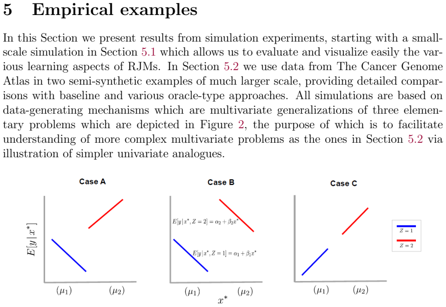
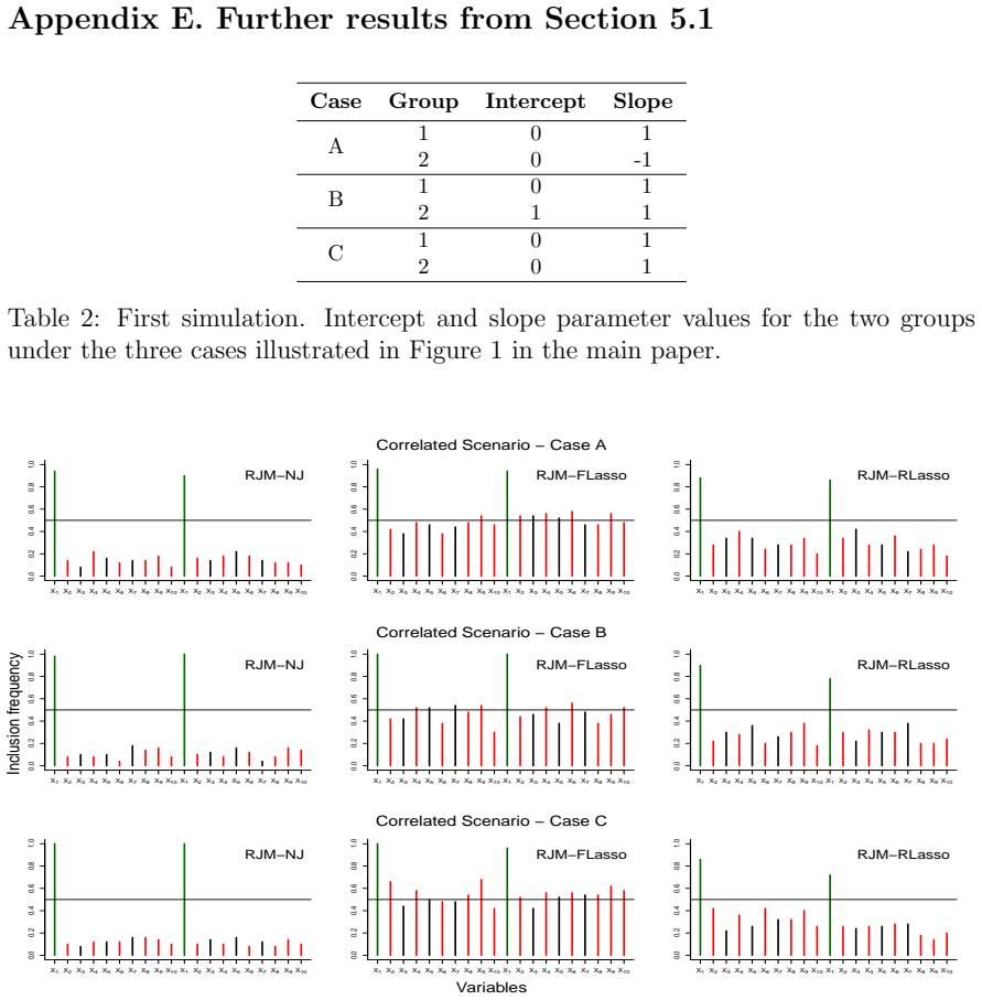
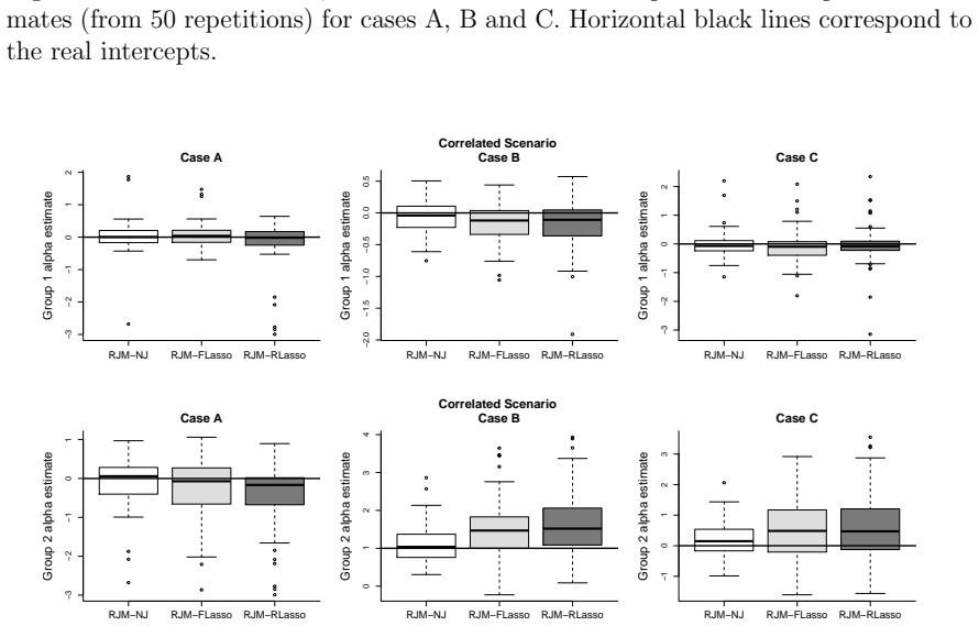
- [Table 2 and Figure 2] Table 2 reports slopes of -1 for both groups under Case A, but Figure 2 and the text describe Case A as having unequal slopes across groups; this is presumably a typographical error in the table but it affects reproducibility of the first simulation.
- [Eq. (37)] In the cluster-selection criterion, the expression X^{*T}_{kg} \hat{\beta}_{kg} appears to have mismatched dimensions if X^* is an n^* by p matrix; it should likely be X^*_{kg} \hat{\beta}_{kg} or the dimensions should be defined consistently.
- [Eq. (13)] The denominator in the E-step formula sums over j but the displayed density inside the sum is written with index k rather than j, which is confusing; the indexing should be corrected for clarity.
- [Figure 8 caption] The caption refers to 'Figure E.7' within a main-text figure; the appendix/figure numbering should be made consistent.
Circularity Check
No significant circularity: the RJM derivation is self-contained; the main caveat is that Theorem 2's penalty condition is not verified for the implemented FLasso/NJ penalties, which is a correctness gap rather than a circular reduction.
full rationale
The paper's derivation chain is not circular. The model, penalties, EM updates, and convergence theorem are constructed explicitly from the likelihood and penalty functions, and no fitted parameter is renamed as a prediction. The RLasso update (22) is an M-step update for the penalty parameter, not a fitted quantity reported as an independent result, and the universal threshold for the graphical lasso is a plug-in tuning choice cited from prior work (Städler and Mukherjee 2013); this self-citation is not load-bearing for the central claim that joint regularized mixture modeling improves upon decoupled or pooled strategies. The main legitimate concern is that Theorem 2's lower-bound condition on the penalty, Eq. (36)/(42), is not satisfied by the implemented negative L1 penalties (FLasso, graphical lasso) or the log|beta| penalty (NJ), and the paper itself excludes only RLasso from the theorem, while the abstract claims convergence is 'established theoretically' without qualification. That is an over-claim or a scope gap in the proof, not a case of the conclusion being equivalent to the inputs by construction. The empirical comparisons are generated from simulations with known ground truth and benchmarked against external methods, so the reported gains are not forced by the model construction. Overall, no circular step of the kind described in the analysis protocol is present.
Assumptions & free parameters
free parameters (4)
- lambda_k (FLasso group penalties) =
Cross-validated, then fixed after assignments stabilize
- c (RLasso prior shape) =
0.25
- zeta (graphical lasso penalty) =
sqrt(2 n log p)/(2 n_k) at each EM step
- K (number of latent groups) =
Selected by predictive loss on held-out data
assumptions (4)
- domain assumption Samples are independent and identically distributed within latent groups
- domain assumption Features X and response Y are normally distributed with identity link
- ad hoc to paper Penalty lower-bound condition (36)/(42) holds
- ad hoc to paper Unique conditional maximization in each block
Cite this review
Pith. "Pith review of Regularized joint mixture models." pith.science (2026). https://pith.science/paper/2GWZ7XT6
@misc{pith2026190807869,
  author       = {Pith},
  title        = {Pith review of: Regularized joint mixture models},
  year         = {2026},
  howpublished = {\url{https://pith.science/paper/2GWZ7XT6}},
  note         = {Machine review of arXiv:1908.07869}
}
read the original abstract
Regularized regression models are well studied and, under appropriate conditions, offer fast and statistically interpretable results. However, large data in many applications are heterogeneous in the sense of harboring distributional differences between latent groups. Then, the assumption that the conditional distribution of response Y given features X is the same for all samples may not hold. Furthermore, in scientific applications, the covariance structure of the features may contain important signals and its learning is also affected by latent group structure. We propose a class of mixture models for paired data (X, Y) that couples together the distribution of X (using sparse graphical models) and the conditional Y | X (using sparse regression models). The regression and graphical models are specific to the latent groups and model parameters are estimated jointly (hence the name "regularized joint mixtures"). This allows signals in either or both of the feature distribution and regression model to inform learning of latent structure and provides automatic control of confounding by such structure. Estimation is handled via an expectation-maximization algorithm, whose convergence is established theoretically. We illustrate the key ideas via empirical examples. An R package is available at https://github.com/k-perrakis/regjmix.
Figures


Figures from the paper (16 more)









Reference graph
Works this paper leans on
-
[1]
Anandkumar, A., Hsu, D. J., Huang, F. and Kakade, S. M. (2012), Learning mixtures of tree graphical models., in ‘NIPS’, pp. 1061–1069. Bae, K. and Mallick, B. (2004), ‘Gene selection using a two-level hierarchical Bayesian model’, Bioinformatics 20, 3423–3430. Banfield, J. D. and Raftery, A. E. (1993), ‘Model-based Gaussian and non-Gaussian clustering’, Bi...
work page 2012
-
[64]
McLachlan, G. and Peel, D. (2000), Finite Mixture Models , John Wiley, New York, USA. McNicholas, D. P. and Murphy, T. B. (2008), ‘Parsimonious Gaussian mixture models’, Statistics and Computing 18(3), 285–296. Meinshausen, N. and B¨ uhlmann, P. (2006), ‘High-dimensional graphs and variable selection with the lasso’, The Annals of Statistics 34, 1436–1462...
arXiv 2000
-
[631]
Friedman, J., Hastie, T. and Tibshirani, R. (2008 a), ‘Regularization paths for general- ized linear models via coordinate descent’,Journal of Statistical Software33(1), 1–22. Friedman, J., Hastie, T. and Tibshirani, R. (2008b), ‘Sparse inverse covariance estima- tion with the graphical lasso’, Biostatistics 9, 432–441. Fr¨ uwirth-Schnatter, S. (2005),Fin...
arXiv 2008
Reviewed August 14, 2026 · model on record in the stance chip above.
Discussion (0). Continue with ORCID to comment.