REVIEW 3 major objections 6 minor 51 references
zELDA II: reconstruction of galactic Lyman-alpha spectra attenuated by the intergalactic medium using neural networks
T0 review · 3 major / 6 minor · reviewed 2026-08-10 · deepseek-v4-flash
Pith's one-line read A neural network can peel the intergalactic medium off Lyman-alpha spectra, recovering the galaxy-emitted line.
desk verdict A solid mock-based method paper whose headline accuracy numbers are properties of the mock generator, not yet the sky; it deserves a serious referee but needs a toned-down abstract or external validation. read the letter →
The pith
A machine-rendered reading of the paper's core claim, the machinery that carries it, and where it could break.
The reading
What carries the argument
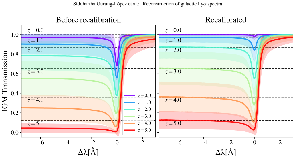
Two precomputed ingredients are combined into training mocks: (i) the 'shell model' grid from the LyaRT Monte Carlo radiative transfer code, a 5D grid over outflow velocity, neutral hydrogen column density, dust optical depth, intrinsic equivalent width, and intrinsic line width that supplies the galaxy-emerging spectrum; and (ii) IGM transmission curves computed from the IllustrisTNG100 simulation, rebinned to continuous redshift by rescaling each snapshot to the mean optical depth of Faucher-Giguère et al. (2008). The networks receive the first 100 PCA components of the observed spectrum plus spectral resolution, pixel size, and (in IGM+z) a proxy redshift; one model (IGM-z) deliberately drops redshift and randomizes the IGM sightlines to avoid imprinting a redshift evolution. The output is the five shell parameters, the true Lyman-alpha wavelength offset, and the IGM Lyman-alpha escape fraction in wavelength windows around line center.
What would settle it
Build a validation set with mock spectra from a different radiative-transfer simulation, such as an ISM model that is not a thin shell or IGM sightlines from a different cosmological simulation, and run zELDA's trained networks on it; if the KS$<0.1$ success fractions or the below-10% transmission uncertainties drop substantially, the in-sample calibration is the cause.
Extended reading notes
Core claim
On the paper's own terms, the discovery is that an observed Lyman-$\alpha$ spectrum contains enough information to recover the pre-IGM ('ISM-emerging') line profile and the line-of-sight IGM escape fraction, provided the training data cover the physical variety of both media. Using a 5D grid of thin-shell outflow parameters for the galaxy and 1000 sightline transmission curves per halo from IllustrisTNG100, the authors train three neural networks; the two that include IGM attenuation (IGM+z and IGM-z) reconstruct the intrinsic line profile with KS$<0.1$ in 95% of COS-like and 80% of MUSE-WIDE-like validation cases, and recover $f^{4\,\text{Å}}_{\mathrm{esc}}$ with typical scatter of about 0.03 for HST-like and 0.12 for MUSE-like spectra. They further show that stacked reconstructed profiles track the true evolution or non-evolution of the intrinsic ISM line with redshift, while a model trained without IGM absorption badly misses the blue peak at high redshift.
Load-bearing premise
Every validation spectrum is made by the same two generators used in training: the LyaRT thin-shell galaxy grid and the IllustrisTNG100 IGM transmission curves, so the accuracy numbers presuppose that these simulations resemble the real ISM and IGM along actual lines of sight.
Editorial extensions
If this is right
- For HST COS-like spectra, zELDA can hand back the intrinsic pre-IGM Lyman-alpha profile for the large majority of sources, enabling studies of ISM outflow properties at redshifts where the IGM previously obscured them.
- Per-source IGM escape fractions allow observers to build Lyman-alpha luminosity functions corrected for IGM attenuation, and to test whether Lyman-alpha visibility depends on large-scale IGM density and velocity fields.
- Reconstructed stacks of ISM-emerging profiles can distinguish true redshift evolution of the galaxy-emerging line from apparent evolution caused by IGM absorption.
- The IGM-z model, designed to be redshift-unbiased, can measure the redshift evolution of the mean IGM escape fraction from z about 2 onward without imposing the training-set redshift dependence.
- For strongly absorbed lines with $f^{4\,\text{Å}}_{\mathrm{esc}}\lesssim0.4$ the reconstruction degrades, so the claimed accuracy applies to the regime where the blue side is not completely erased.
Reading between the lines
- The headline accuracy numbers are measured on validation mocks built with the same forward models used to train the networks, so they quantify in-sample inversion performance rather than guaranteed performance on real observed spectra.
- A direct observational test would be to compare zELDA's per-source escape fractions with IGM transmission measured independently along the same sightlines, for example using background quasars or close pairs of galaxies.
- If real ISM geometries deviate from the thin-shell model, the recovered intrinsic profiles could be the best shell-model projection rather than the true spectrum; retraining or validating on non-shell radiative transfer outputs would reveal the size of this effect.
- The same PCA-plus-neural-network scheme could be adapted to other resonant lines or to jointly fitting Lyman-alpha with UV continuum information to break remaining degeneracies between outflow parameters and IGM absorption.
Editorial analysis
A structured set of objections, weighed in public.
Referee Report
Summary. The paper presents zELDA II, an open-source Python module that uses artificial neural networks to disentangle the interstellar medium (ISM) and intergalactic medium (IGM) contributions to observed Lyα spectra. Mock spectra are generated by convolving LyaRT 'thin shell' profiles (the zELDA I forward model) with IGM transmission curves from Byrohl & Gronke (2020) (IllustrisTNG100), downgraded to various spectral resolutions and signal-to-noise ratios. Three network variants are trained: IGM+z (input includes proxy redshift, IGM curves assigned at the source redshift), IGM-z (no redshift input, randomized IGM curves), and NoIGM (no IGM attenuation during training). The networks output shell parameters, redshift offset, and IGM escape fractions f_xÅ_esc. The paper reports that on mock spectra, IGM+z and IGM-z reconstruct intrinsic profiles with KS<0.1 for 95% (HST/COS-like) and ~80% (MUSE-WIDE-like) of cases, and measure f^4Å_esc with 'typical uncertainties below 10%' (abstract) or ~0.12 (Sect. 5). The paper also tests recovery of prescribed mean f_esc evolutions and stacked line profiles. Public code and documentation are provided.
Significance. If the quoted accuracies were validated on independent data, the method would be a valuable tool for separating ISM and IGM effects in Lyα spectroscopy and for deriving IGM escape fractions source-by-source. The paper strengthens the earlier zELDA framework with a PCA-based input representation and several carefully compared network models, and it provides reproducible code, extensive accuracy tables (Appendices C-D), and an honest uncertainty-calibration analysis (Appendix B). The main caveat is that all quantitative performance claims are measured on mock spectra generated by the same forward model used to construct the training set; the reported 95%/80% success fractions and sub-10% f_esc uncertainties are therefore properties of the mock generator rather than demonstrated properties of real observations. The abstract does not make this limitation clear.
major comments (3)
- [Sects. 2.3, 3.2, 4; Appendices C-D] The validation is in-sample. The training set (Sect. 3.2) and the mock validation set (Sect. 4; Appendices C-D) are generated by the same forward model: LyaRT thin-shell profiles (Sect. 2.1) convolved with Byrohl & Gronke (2020) IllustrisTNG100 IGM transmission curves (Sect. 2.2), then degraded to the same observational configurations. The networks therefore learn and are tested on the same distribution. The paper states (Sect. 5) that 'we have tested our ANN models in mock Lyα line profiles' and then reports the 95%/80% KS<0.1 fractions and ~0.03/~0.12 f_esc uncertainties as if they apply to observed data, but no test on observed spectra or on an independent forward model is presented. This is load-bearing for the central claim that zELDA can reconstruct ISM-emerging Lyα profiles of observed galaxies. I request either a demonstration on real data (even a small pilot sample of COS/MUSE spectra), a validation against a forward model not used in training (e.g., an alternative IGM simulation or a non-shell ISM geometry), or an explicit qualification in the abstract and conclusions that these accuracy numbers are in-sample mock validation results. The 'redshift-unbiased' design of IGM-z does not remove this dependence, because both training and test IGM curves are drawn from the same IllustrisTNG100-based set.
- [Abstract; Sect. 5; Fig. C.2] The abstract's claim that zELDA measures the IGM transmission 'with typical uncertainties below 10% for HST-COS and MUSE-WIDE data' is not supported by the body. Section 5 reports f^4Å_esc uncertainties of ~0.03 for HST-like and ~0.12 for MUSE-like data, and Fig. C.2 (IGM-z, f^4Å_esc bins) shows accuracies of 0.08-0.16 for Wg=2.0 Å (MUSE-like) across the f_esc range, with values above 0.10 for most f_esc bins. Please reconcile the abstract with the tabulated values and avoid stating 'below 10%' for MUSE-WIDE-like data unless a stricter subset (e.g., only f_esc>0.8) is explicitly defined.
- [Sect. 4.2.1, Eq. (3)] The f_esc evolution tests are constructed by prescribing the mean f_esc as a Fermi-Dirac function of redshift and then drawing IGM transmission curves until the computed f_esc lies within 10% of the prescribed ⟨f_esc⟩. Recovering this prescribed trend with the network shows that the network can invert the training distribution, but it does not independently verify the ability to measure the true IGM transmission evolution. Statements such as 'IGM+z and IGM-z are able to detect evolution in f_esc from redshift 2.0 onward for MUSE-like data' (Sect. 5) should be explicitly labeled as tests on mocks with injected evolution; as written, they overstate the evidence.
minor comments (6)
- [Throughout] The spelling 'Kolmogórov-Smirnov' appears in several places (e.g., abstract, Sect. 4.1, Appendix D); the standard spelling is 'Kolmogorov-Smirnov'.
- [Fig. 4 caption] The caption says 'Ly α line profiles spamming zELDA's grid'; 'spamming' should be 'spanning'.
- [References] The entries Gurung-López et al. 2021a and 2021b share the same volume/page (MNRAS, 500, 603); please check whether one of these is a different article (and cite accordingly in the text).
- [Sect. 3.4] The sentence 'For each output property, we trained an independent ANN' is clear, but the training set sizes and the convergence test ('We tested that for this training set size, our artificial neural networks have converged') are not quantified; adding a brief description (e.g., loss curves or a convergence criterion) would improve reproducibility.
- [Sect. 2.1] The parameter range for τ_a is printed as 'τa∈ [0.0001, 0.0]' in the text; this appears to be a typo, since dust optical depth τ_a=0.0 would make the lower bound meaningless. Please verify and correct.
- [Fig. D.1] The x-axis label 'log KS' is ambiguous: it is not clear whether the base is 10 and whether KS is the standard Kolmogorov-Smirnov statistic; please state 'log10 KS'.
Circularity Check
No circularity: the accuracy claims are measured on held-out mocks from the same forward model used for training, which is a limitation on external validity but not a logically circular derivation.
full rationale
The claimed derivation chain is: generate mock Lyα spectra by convolving LyaRT thin-shell profiles (Sect. 2.1, from the authors' ZP22 grid) with Byrohl & Gronke (2020) IllustrisTNG100 IGM transmission curves (Sect. 2.2), train artificial neural networks to map those mock observed spectra to shell parameters, redshift, and f_esc (Sect. 3), and then evaluate on held-out mocks produced by the same generator (Sect. 4 and Appendices C-D). This is an in-sample evaluation: the reported KS and f_esc accuracies quantify how well the networks invert their own training forward model, and they do not by themselves establish performance on real spectra if the true ISM or IGM departs from the thin-shell model or from IllustrisTNG100. That is a genuine external-validity limitation, and the paper is largely transparent that all accuracy results are on mock line profiles. It is not a circular derivation under the seven enumerated patterns: the validation mocks are not used to set the network weights, the networks demonstrably fail on identifiable subsets (e.g., low f_esc, and NoIGM at high redshift), and the f_esc-evolution tests in Sect. 4.2 are injection-recovery checks where the truth is imposed by a Fermi-Dirac rejection procedure and then independently estimated, with reported biases rather than tautological agreement. The self-citations (ZP22 and Byrohl & Gronke 2020) supply the forward model and are externally published, based on public codes and simulations, and falsifiable against Lyα observations; they are not invoked as uniqueness theorems or to forbid alternatives. One non-circular inconsistency exists: the abstract states typical MUSE-WIDE IGM transmission uncertainties below 10%, while Sect. 5 and Appendix C report about 0.12 in the MUSE-like regime; this affects the consistency of the claims, not the logical structure of the derivation. No circular step meets the evidence bar.
Assumptions & free parameters
free parameters (6)
- KS success threshold =
0.1
- Number of PCA components =
100
- ANN architecture =
Three-layer (103, 53, 25) for most outputs; nine-layer for Delta_lambda_True
- Training set size =
4.5e6
- f_esc wavelength window =
4 Angstrom
- Fermi-Dirac mock parameters a and b =
Mock1 {7.0, 0.7}, Mock2 {6.0, 0.6}, Mock3 {5.0, 0.5}, Mock4 {4.0, 0.4}
assumptions (7)
- domain assumption Thin shell model with parameters Vexp, NH, tau_a, EWin, Win describes the ISM-emerging Ly-alpha profile.
- domain assumption Byrohl & Gronke (2020) IGM transmission curves from IllustrisTNG100 span the real diversity of IGM attenuation.
- domain assumption Faucher-Giguere et al. (2008) mean optical depth evolution is correct and can rescale snapshot curves.
- domain assumption Observed Ly-alpha spectrum = intrinsic profile multiplied by IGM transmission, then convolved with instrument Gaussian and pixelated, plus Gaussian noise.
- ad hoc to paper ANNs trained on this forward model generalize to real observed Ly-alpha spectra.
- domain assumption The 100 PCA components retain the information needed for parameter inference.
- domain assumption The observed global maximum wavelength is a usable redshift proxy.
Cite this review
Pith. "Pith review of zELDA II: reconstruction of galactic Lyman-alpha spectra attenuated by the intergalactic medium using neural networks." pith.science (2026). https://pith.science/paper/2OZOWJPF
@misc{pith2026250104077,
  author       = {Pith},
  title        = {Pith review of: zELDA II: reconstruction of galactic Lyman-alpha spectra attenuated by the intergalactic medium using neural networks},
  year         = {2026},
  howpublished = {\url{https://pith.science/paper/2OZOWJPF}},
  note         = {Machine review of arXiv:2501.04077}
}
read the original abstract
The observed Lyman-Alpha (Lya) line profile is a convolution of the complex Lya radiative transfer taking place in the interstellar, circumgalactic and intergalactic medium (ISM, CGM, and IGM, respectively). Discerning the different components of the Lya line is crucial in order to use it as a probe of galaxy formation or the evolution of the IGM. We present the second version of zELDA (redshift Estimator for Line profiles of Distant Lyman-Alpha emitters), an open-source Python module focused on modeling and fitting observed Lya line profiles. This new version of zELDA focuses on disentangling the galactic from the IGM effects. We build realistic Lya line profiles that include the ISM and IGM contributions, by combining the Monte Carlo radiative transfer simulations for the so called "shell model" (ISM) and IGM transmission curves generated from IllustrisTNG100. We use these mock line profiles to train different artificial neural networks. These use as input the observed spectrum and output the outflow parameters of the best fitting "shell model" along with the redshift and Lya emission IGM escape fraction of the source. We measure the accuracy of zELDA on mock Lya line profiles. We find that zELDA is capable of reconstructing the ISM emerging Lya line profile with high accuracy (Kolmogorov-Smirnov<0.1) for 95% of the cases for HST COS-like observations and 80% for MUSE-WIDE-like. zELDA is able to measure the IGM transmission with the typical uncertainties below 10% for HST-COS and MUSE-WIDE data. This work represents a step forward in the high-precision reconstruction of IGM attenuated Lya line profiles. zELDA allows the disentanglement of the galactic and IGM contribution shaping the Lya line shape, and thus allows us to use Lya as a tool to study galaxy and ISM evolution.
Figures


Figures from the paper (9 more)


Reference graph
Works this paper leans on
-
[1]
, " * write output.state after.block = add.period write newline
ENTRY address archiveprefix author booktitle chapter edition editor howpublished institution eprint journal key month note number organization pages publisher school series title type volume year label extra.label sort.label short.list INTEGERS output.state before.all mid.sentence after.sentence after.block FUNCTION init.state.consts #0 'before.all := #1 ...
-
[2]
write newline
" write newline "" before.all 'output.state := FUNCTION n.dashify 't := "" t empty not t #1 #1 substring "-" = t #1 #2 substring "--" = not "--" * t #2 global.max substring 't := t #1 #1 substring "-" = "-" * t #2 global.max substring 't := while if t #1 #1 substring * t #2 global.max substring 't := if while FUNCTION word.in bbl.in " " * FUNCTION format....
-
[3]
2003, Journal of Korean Astronomical Society, 36, 145
Ahn , S. 2003, Journal of Korean Astronomical Society, 36, 145
work page 2003
-
[4]
Behrens , C., Pallottini , A., Ferrara , A., Gallerani , S., & Vallini , L. 2019, , 486, 2197
work page 2019
- [5]
- [6]
- [7]
- [8]
Show all 51 references
-
[9]
2006, , 649, 14
Dijkstra , M., Haiman , Z., & Spaans , M. 2006, , 649, 14
2006
-
[10]
J., S \'a nchez , A
Farrow , D. J., S \'a nchez , A. G., Ciardullo , R., et al. 2021, arXiv e-prints, arXiv:2104.04613
2021 arXiv
-
[11]
X., Lidz , A., Hernquist , L., & Zaldarriaga , M
Faucher-Gigu \`e re , C.-A., Prochaska , J. X., Lidz , A., Hernquist , L., & Zaldarriaga , M. 2008, , 681, 831
2008
-
[12]
C., Froning , C
Green , J. C., Froning , C. S., Osterman , S., et al. 2012, , 744, 60
2012
-
[13]
2022, arXiv e-prints, arXiv:2206.14908
Greene , J., Bezanson , R., Ouchi , M., Silverman , J., & the PFS Galaxy Evolution Working Group . 2022, arXiv e-prints, arXiv:2206.14908
2022 arXiv
-
[14]
2017, , 608, A139
Gronke , M. 2017, , 608, A139
2017
-
[15]
Gronke , M., Dijkstra , M., McCourt , M., & Oh , S. P. 2016, , 833, L26
2016
-
[16]
Gurung-L \'o pez , S., Gronke , M., Saito , S., Bonoli , S., & Orsi , \'A . A. 2022, , 510, 4525
2022
-
[17]
A., & Bonoli , S
Gurung-L \'o pez , S., Orsi , \'A . A., & Bonoli , S. 2019 a , , 490, 733
2019
-
[18]
A., Bonoli , S., Baugh , C
Gurung-L \'o pez , S., Orsi , \'A . A., Bonoli , S., Baugh , C. M., & Lacey , C. G. 2019 b , , 486, 1882
2019
-
[19]
A., Bonoli , S., et al
Gurung-L \'o pez , S., Orsi , \'A . A., Bonoli , S., et al. 2020, , 491, 3266
2020
-
[20]
M., et al
Gurung-L \'o pez , S., Saito , S., Baugh , C. M., et al. 2021 a , , 500, 603
2021
-
[21]
M., et al
Gurung-L \'o pez , S., Saito , S., Baugh , C. M., et al. 2021 b , , 500, 603
2021
-
[22]
R., Millman, K
Harris, C. R., Millman, K. J., van der Walt, S. J., et al. 2020, Nature, 585, 357
2020
-
[23]
J., Runnholm , A., Scarlata , C., Gronke , M., & Rivera-Thorsen , T
Hayes , M. J., Runnholm , A., Scarlata , C., Gronke , M., & Rivera-Thorsen , T. E. 2023, , 520, 5903
2023
-
[24]
C., Urrutia , T., Wisotzki , L., et al
Herenz , E. C., Urrutia , T., Wisotzki , L., et al. 2017, , 606, A12
2017
-
[25]
J., Gebhardt , K., Komatsu , E., et al
Hill , G. J., Gebhardt , K., Komatsu , E., et al. 2008, in Astronomical Society of the Pacific Conference Series, Vol. 399, Astronomical Society of the Pacific Conference Series, ed. T. Kodama, T. Yamada, & K. Aoki , 115--+
2008
-
[26]
Hunter, J. D. 2007, Computing In Science & Engineering, 9, 90
2007
-
[27]
2019, arXiv e-prints, arXiv:1906.00173
Kakuma , R., Ouchi , M., Harikane , Y., et al. 2019, arXiv e-prints, arXiv:1906.00173
2019 arXiv
-
[28]
Laursen , P., Sommer-Larsen , J., & Razoumov , A. O. 2011, , 728, 52
2011
-
[29]
2018, , 480, 5113
Marinacci , F., Vogelsberger , M., Pakmor , R., et al. 2018, , 480, 5113
2018
-
[30]
P., Pillepich , A., Springel , V., et al
Naiman , J. P., Pillepich , A., Springel , V., et al. 2018, , 477, 1206
2018
-
[31]
2019, Computational Astrophysics and Cosmology, 6, 2
Nelson , D., Springel , V., Pillepich , A., et al. 2019, Computational Astrophysics and Cosmology, 6, 2
2019
-
[32]
Neufeld , D. A. 1990, , 350, 216
1990
-
[33]
G., & Baugh , C
Orsi , A., Lacey , C. G., & Baugh , C. M. 2012, , 425, 87
2012
-
[34]
2014, , 443, 799
Orsi , \'A ., Padilla , N., Groves , B., et al. 2014, , 443, 799
2014
-
[35]
2018, , 70, S13
Ouchi , M., Harikane , Y., Shibuya , T., et al. 2018, , 70, S13
2018
-
[36]
2020, Annual Review of Astronomy and Astrophysics, 58, 617
Ouchi, M., Ono, Y., & Shibuya, T. 2020, Annual Review of Astronomy and Astrophysics, 58, 617
2020
-
[37]
2018, , 475, 648
Pillepich , A., Nelson , D., Hernquist , L., et al. 2018, , 475, 648
2018
-
[38]
C., Steidel , C
Rudie , G. C., Steidel , C. C., & Pettini , M. 2012, , 757, L30
2012
-
[39]
2021, , 133, 034507
Runnholm , A., Gronke , M., & Hayes , M. 2021, , 133, 034507
2021
-
[40]
2011, , 531, A12
Schaerer , D., Hayes , M., Verhamme , A., & Teyssier , R. 2011, , 531, A12
2011
-
[41]
2020, , 643, A149
Spinoso , D., Orsi , A., L \'o pez-Sanjuan , C., et al. 2020, , 643, A149
2020
-
[42]
2018, , 475, 676
Springel , V., Pakmor , R., Pillepich , A., et al. 2018, , 475, 676
2018
-
[43]
C., Erb , D
Steidel , C. C., Erb , D. K., Shapley , A. E., et al. 2010, , 717, 289
2010
-
[44]
2023, , 680, A14
Torralba-Torregrosa , A., Gurung-L \'o pez , S., Arnalte-Mur , P., et al. 2023, , 680, A14
2023
-
[45]
2024, , 690, A388
Torralba-Torregrosa , A., Renard , P., Spinoso , D., et al. 2024, , 690, A388
2024
-
[46]
2019, , 624, A141
Urrutia , T., Wisotzki , L., Kerutt , J., et al. 2019, , 624, A141
2019
-
[47]
2018, , 478, L60
Verhamme , A., Garel , T., Ventou , E., et al. 2018, , 478, L60
2018
-
[48]
2007, in Astronomical Society of the Pacific Conference Series, Vol
Verhamme , A., Schaerer , D., Atek , H., & Tapken , C. 2007, in Astronomical Society of the Pacific Conference Series, Vol. 380, Deepest Astronomical Surveys, ed. J. Afonso , H. C. Ferguson , B. Mobasher , & R. Norris , 97
2007
-
[49]
E., et al
Virtanen , P., Gommers , R., Oliphant , T. E., et al. 2020, Nature Methods, 17, 261
2020
-
[50]
H., Bowman , W
Weiss , L. H., Bowman , W. P., Ciardullo , R., et al. 2021, , 912, 100
2021
-
[51]
2011, , 726, 38
Zheng , Z., Cen , R., Trac , H., & Miralda-Escud \'e , J. 2011, , 726, 38
2011
Reviewed August 10, 2026 · model on record in the stance chip above.
Discussion (0). Continue with ORCID to comment.