REVIEW 4 major objections 5 minor 44 references
Validating time-distance helioseismic inversions for non-separable subsurface profiles of an average supergranule
T0 review · 4 major / 5 minor · reviewed 2026-08-14 · deepseek-v4-flash
Pith's one-line read Time-distance helioseismic inversions recover the peak depth of non-separable supergranule models, even when the full subsurface flow is not retrieved.
desk verdict A careful, honest validation showing that peak depth, not the full flow, is recoverable for non-separable supergranule models; the noise-free setup keeps the claim modest but leaves the abstract's 'above noise cutoff' untested. read the letter →
The pith
A machine-rendered reading of the paper's core claim, the machinery that carries it, and where it could break.
The reading
What carries the argument
The central object is the stream function $\psi(x,z)$ that generates a mass-conserving flow through $\mathbf{v} = \rho^{-1}\nabla\times(\rho\psi\,\hat{\mathbf{y}})$. It is written as a weighted sum over normalized Legendre polynomials in the horizontal direction and expanded on cubic B-splines in the vertical direction, which encodes an implicit smoothness regularization and shrinks the parameter count from a full gridded flow to hundreds or thousands of coefficients. The inversion iteratively updates only the subsurface B-spline coefficients, while the coefficients at and above the surface are fixed to their true values. The gradient direction comes from adjoint sensitivity kernels, $K_{i\ell}=\int dx\,K_\psi(x)B_i(z)f_\ell(x)$, and the optimization is carried out with BFGS or nonlinear conjugate gradients, minimizing the squared travel-time misfit between true and iterated models.
What would settle it
Run the same four depth-peaking models with realistic noise added to the surface Doppler velocities, or with the surface coefficients estimated from the data rather than fixed to their true values, and record how often the recovered peak depth stays within the spread of Fig. 6; if modest noise pushes the inferred peak depth away from the true value, the claim that peak depth is reliably recoverable fails.
Extended reading notes
Core claim
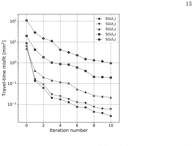
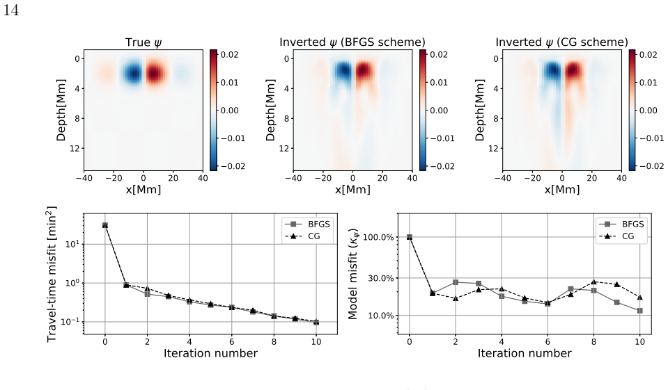
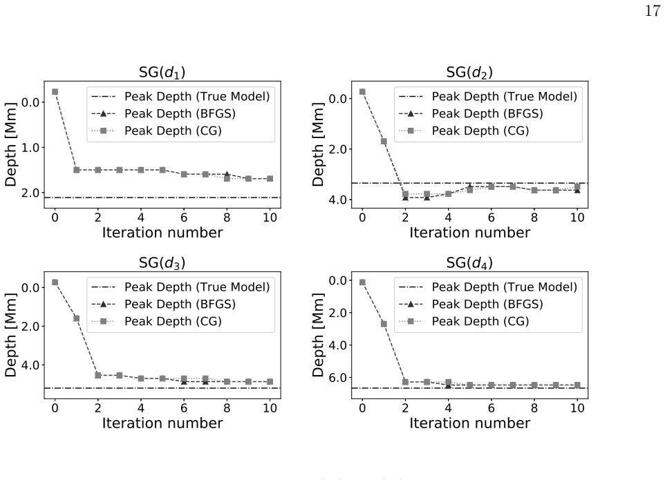
The paper claims that with the chosen implicit regularization, travel-time inversions of non-separable supergranule models recover their peak depths accurately even though the full velocity field is not recovered. For the low-dimensional case, with fewer than roughly 200 parameters, the iterative inversion approaches the true flow; for larger models the travel-time misfit keeps falling but the solution converges to a local minimum. In all depth-peaking models SG(d1)-SG(d4), the peak depth of the horizontally averaged squared stream function is retrieved within roughly two iterations, using either BFGS or conjugate-gradient optimization. The paper defines this peak depth as a lower-bound estimator of supergranule depth and argues the result is an important step toward identifying what can be reliably inferred from time-distance helioseismology.
Load-bearing premise
The inversion fixes the stream-function coefficients at and above the solar surface to their true values (Eqs. 6-7), so the algorithm is handed the exact surface flow and only needs to find the subsurface part; noisy or biased surface measurements could destroy the peak-depth recovery.
Editorial extensions
If this is right
- Peak depth is a robust inferential target: even when the inversion falls into a local minimum, the depth of maximum $\int\psi^2\,dx$ comes out right in about two iterations.
- For flows described by fewer than about 200 parameters, the full stream function and velocity components are progressively recovered, suggesting that smaller basis sets are a route to full-profile inversions.
- The monotonically decreasing travel-time misfit in high-dimensional runs is not evidence of convergence to the true model, since the model misfit can worsen while travel-time misfit improves.
- Ensemble averaging over supergranule cells, which improves signal-to-noise by roughly $\sqrt{N}$, may allow the depth recovery demonstrated here to be translated into bounds on real supergranule depths.
- Depth estimates obtained this way can be compared with mode-coupling and holographic estimates to check consistency among helioseismic techniques.
Reading between the lines
- If the peak-depth recovery is as robust in the presence of noise as it is here, then depth becomes a practical observable for testing supergranule formation theories, such as rotation-suppression or shallow-convection models.
- The surface coefficients fixed in Eqs. (6)-(7) are an optimistic premise; a test with noisy or estimated surface velocities is the natural next validation, and the paper itself notes that noise will limit how deeply the kernels can probe.
- The local-minimum behaviour suggests that travel-time misfit alone is a weak selector among high-dimensional flow models; adding model-covariance or prior information, as the authors note, could turn the recovered depth into a full profile with uncertainties.
- One could test whether the same basis regularization recovers peak depth for non-axisymmetric or time-dependent supergranules, since the present models are azimuthally symmetric and stationary.
Signed reviews
Editorial analysis
A structured set of objections, weighed in public.
Referee Report
Summary. The paper presents synthetic validation tests of time-distance helioseismic inversions for non-separable models of an average supergranule. The flow is written as a sum of Gaussians in depth times Legendre polynomials in the horizontal coordinate, projected onto a B-spline basis. Travel times and sensitivity kernels are computed with the SPARC code, and BFGS and conjugate-gradient optimizers update the subsurface B-spline coefficients to minimize a travel-time misfit. For low-dimensional models (69-161 parameters) the flow profile approaches the truth; for high-dimensional models the exact profile is not recovered, but the peak depth, defined by the maximum of the horizontally averaged squared stream function, is recovered within about two iterations for four models peaking at different depths. All experiments are noise-free and the surface stream-function coefficients are fixed to their true values.
Significance. If the result holds, it is a meaningful step: it extends earlier separable-profile inversions (Bhattacharya et al. 2017) to non-separable models, uses a consistent forward-plus-adjoint framework in the public SPARC code, and cross-validates the BFGS and CG optimizers. The recovery of a depth scale despite failure to recover the full profile is a falsifiable, practically useful outcome. However, the headline claim is currently conditional on two untested idealizations, exact surface flow and noise-free travel times, so the significance is moderate until those gaps are addressed.
major comments (4)
- [Section 2.2, Eqs. (6)-(7)] The inversion fixes all B-spline coefficients at and above the surface to their true values, so the surface velocity is exactly known. This is a strong assumption that is not available in practice: real HMI-style Doppler measurements carry realization noise, and an ensemble-averaged supergranule surface profile has its own bias and uncertainty. Since the central claim concerns recovering peak depth from measurements 'presumably above the noise cutoff,' the paper needs to test robustness to perturbed or co-inverted surface coefficients and to noisy travel times before that claim can be considered established.
- [Section 4 and Section 5, Figs. 3-4] All inversions are noise-free: the misfit in Eq. (9) compares exact synthetic travel times, and no realization noise, data covariance, or measurement uncertainties are introduced. The abstract's hedge 'presumably above the noise cutoff' is therefore not actually tested. The conclusion itself concedes that uncertainties are lacking and that the noisy-measurement case requires further work; that concession should move into the central validation, for example by adding noise at levels typical of HMI ensemble-averaged supergranule measurements and recomputing peak-depth recovery. Without such experiments, the headline result remains conditional.
- [Section 4.2, Eq. (13)] The peak depth is computed from the horizontally averaged squared stream function of the same B-spline/Legendre representation used in the inversion. Because the surface coefficients are fixed to truth and the B-spline basis is smooth, the depth estimator may inherit information from the prior and the basis rather than from the travel-time data. The paper would be strengthened by a control experiment using a different basis for the inversion or a different, more model-independent definition of depth, such as the depth of maximum vertical velocity, to confirm that the travel-time data alone carry the depth information. This is important because Fig. 2 shows that for models with many parameters the inverted flow profile is not close to the true model, yet the peak depth is recovered.
- [Section 4.1, Figs. 2-3 and Section 4.2, Figs. 5-7] For models SG(l3)-SG(l5), the model misfit kappa increases while the travel-time misfit decreases, which the authors interpret as convergence to local minima. If the same local-minimum behavior occurs in Case 2, the recovered peak depth could be a property of the starting model and basis rather than of the data. Please report the travel-time misfit and model-misfit curves for the SG(d1)-SG(d4) inversions and test whether the recovered peak depth depends on the starting model, for example by starting from a nonzero subsurface flow with a different initial depth.
minor comments (5)
- [Section 3, Eq. (8)] Equation (8) appears to contain a typo in the advection term: the term 2 rho v . grad partial_t^2 xi should likely be 2 rho v . grad partial_t xi, since the dimensions otherwise do not match the other terms. Please verify and correct the equation or explain the notation.
- [Figures 2 and 4] Several figure labels are corrupted or misspelled: 'De th[Mm]', 'In%erted', and 'In)erted' should read 'Depth [Mm]' and 'Inverted'. The figures should be regenerated with correct labels.
- [Figure 6] The axes in Fig. 6 are inverted so that larger depths appear to the left, and the panels lack axis labels and quantitative error bars or scatter estimates; please consider using a standard depth axis with depth increasing downward and adding labels or a caption note explaining the orientation.
- [Section 5, Conclusion] The statement that inversions 'are able to recover their peak depths accurately' should be qualified to indicate that this is demonstrated for noise-free synthetic data with exactly known surface boundary conditions; the current wording overstates what the experiments show.
- [Abstract and Introduction] The phrase 'presumably above the noise cutoff' in the abstract is a hedge that belongs in the results or conclusion rather than in the abstract, since no noise cutoff is computed or applied anywhere in the paper.
Circularity Check
No significant circularity: peak-depth recovery is an emergent inversion outcome, not a fitted input.
full rationale
The paper performs a self-contained synthetic validation. The true stream function is constructed (Eq. 3), travel times are forward-modelled (Eqs. 8-9), adjoint sensitivity kernels are computed (Eqs. 10-11), and the subsurface B-spline coefficients are iteratively updated. The reported peak depth (Eq. 13) is an output of the optimized stream function, not a parameter that was fitted to its own target value. Fixing the surface coefficients to the true values (Eqs. 6-7) is a stated simplifying assumption, and it weakens the realism of the validation, but it does not make the subsurface peak-depth recovery equivalent to the inputs by construction. The reliance on prior work by the same authors concerns the inversion methodology and basis choice, not an unverified theorem on which the central claim rests. The paper's own conclusion concedes that noisy measurements and uncertainty estimates are not addressed, which is a scope limitation rather than a circular step. No specific reduction of a prediction to its fitted input or to a self-citation chain can be exhibited.
Assumptions & free parameters
free parameters (3)
- Gaussian alpha_l distribution (peak l=121, sigma_l, v0) =
sigma_l = 1,4,10,25; v0 = 200-550 m/s (Table 1)
- Subsurface B-spline coefficients (69-2400 per model) =
Final values from BFGS/CG optimization (not tabulated)
- Model length scales R and k =
R = 10 Mm, k = 2*pi/30 Mm^-1
assumptions (6)
- domain assumption The wave equation (Eq. 8) and SPARC code accurately model solar acoustic wave propagation through supergranule flows.
- domain assumption The travel-time measurement technique (Gizon & Birch 2002, ridge filtering) provides a faithful observable for the inversion.
- domain assumption The average supergranule is azimuthally symmetric, reducing the problem to 2D.
- domain assumption The stream function is representable in the chosen Legendre/B-spline basis, and the true model lies within the inversion's model space.
- ad hoc to paper The surface stream function coefficients are exactly known and fixed to the true model (Eqs. 6-7).
- ad hoc to paper The peak depth of the horizontally averaged squared stream function (Eq. 13) is a meaningful estimator of supergranule depth.
Cite this review
Pith. "Pith review of Validating time-distance helioseismic inversions for non-separable subsurface profiles of an average supergranule." pith.science (2026). https://pith.science/paper/2PVJNTFF
@misc{pith2026190808456,
  author       = {Pith},
  title        = {Pith review of: Validating time-distance helioseismic inversions for non-separable subsurface profiles of an average supergranule},
  year         = {2026},
  howpublished = {\url{https://pith.science/paper/2PVJNTFF}},
  note         = {Machine review of arXiv:1908.08456}
}
read the original abstract
Supergranules are divergent 30-Mm sized cellular flows observed everywhere at the solar photosphere. Their place in the hierarchy of convective structures and their origin remain poorly understood (Rincon et al., 2018). Estimating supergranular depth is of particular interest since this may help point to the underlying physics. However, their subsurface velocity profiles have proven difficult to ascertain. Birch et al. (2006) had suggested that helioseismic inferences would benefit from an ensemble average over multiple realizations of supergranules due to the reduction in realization noise. Bhattacharya et al. (2017) used synthetic forward-modelled seismic wave travel times and demonstrated the potential of helioseismic inversions at recovering the flow profile of an average supergranule that is separable in the horizontal and vertical directions, although the premise of this calculation has since been challenged by Ferret (2019). In this work we avoid this assumption and carry out a validation test of helioseismic travel-time inversions starting from plausible synthetic non-separable profiles of an average supergranule. We compute seismic wave travel times and sensitivity kernels by simulating wave propagation through this background. We find that, while the ability to recover the exact profile degrades based on the number of parameters involved, we are nevertheless able to recover the peak depth of our models in a few iterations where the measurements are presumably above the noise cutoff. This represents an important step towards unraveling the physics behind supergranules, as we start appreciating the parameters that we may reliably infer from a time-distance helioseismic inversion.
Figures


Figures from the paper (4 more)


Reference graph
Works this paper leans on
-
[1]
Bhattacharya, J., & Hanasoge, S. M. 2016, ApJ, 826, 105, doi: 10.3847/0004-637X/826/2/105
-
[2]
2017, A&A, 607, A129, doi: 10.1051/0004-6361/201731095
Gizon, L. 2017, A&A, 607, A129, doi: 10.1051/0004-6361/201731095
-
[3]
L., Gizon, L., & Jackiewicz, J
Birch, A., Duvall, T. L., Gizon, L., & Jackiewicz, J. 2006, in AAS/Solar Physics Division Meeting #37, AAS/Solar Physics Division Meeting, 5.05
work page 2006
-
[4]
Braun, D. C., Birch, A. C., Benson, D., Stein, R. F., & Nordlund, Å. 2007, ApJ, 669, 1395, doi: 10.1086/521782
-
[5]
Braun, D. C., Birch, A. C., & Lindsey, C. 2004, in ESA Special Publication, Vol. 559, SOHO 14 Helio- and Asteroseismology: Towards a Golden Future, ed. D. Danesy, 337
work page 2004
- [6]
-
[7]
D., Charbonneau, P., & Thibault, K
Crouch, A. D., Charbonneau, P., & Thibault, K. 2007, ApJ, 662, 715, doi: 10.1086/515564
-
[8]
2015, SoPh, 290, 1547, doi: 10.1007/s11207-015-0693-0 Del Moro, D
DeGrave, K., & Jackiewicz, J. 2015, SoPh, 290, 1547, doi: 10.1007/s11207-015-0693-0 Del Moro, D. 2004, A&A, 428, 1007, doi: 10.1051/0004-6361:20040466
Show all 44 references
-
[9]
Hanasoge, S. M. 2013, Solar Physics, 282, 361, doi: 10.1007/s11207-012-0189-0
2013 doi
-
[10]
Duvall, J., & Birch, A. C. 2010, ApJ, 725, L47, doi: 10.1088/2041-8205/725/1/L47
2010 doi
-
[11]
2012, SoPh, 136, doi: 10.1007/s11207-012-0010-0
Duvall, T., & Hanasoge, S. 2012, SoPh, 136, doi: 10.1007/s11207-012-0010-0
2012 doi
-
[12]
Duvall, Jr., T. L. 1998, in ESA Special
1998
-
[13]
A., & Hindman, B
Featherstone, N. A., & Hindman, B. W. 2016, ApJL, 830, L15, doi: 10.3847/2041-8205/830/1/L15
2016 doi
-
[14]
Ferret, R. Z. 2019, A&A, 623, doi: 10.1051/0004-6361/201833742
2019 doi
-
[15]
Gizon, L., & Birch, A. C. 2002, ApJ, 571, 966, doi: 10.1086/340015
2002 doi
-
[16]
Gizon, L., & Duvall, T. L. 2004, in IAU
2004
-
[17]
L., & Schou, J
Gizon, L., Duvall, T. L., & Schou, J. 2003, Nature, 421, 43, doi: 10.1038/nature01287
2003 doi
-
[18]
J., Hindman, B
Greer, B. J., Hindman, B. W., & Toomre, J. 2016, ApJ, 824, 128, doi: 10.3847/0004-637X/824/2/128
2016 doi
-
[19]
Hanasoge, S. M. 2014, ApJ, 797, 23, doi: 10.1088/0004-637X/797/1/23
2014 doi
-
[20]
M., Birch, A., Gizon, L., & Tromp, J
Hanasoge, S. M., Birch, A., Gizon, L., & Tromp, J. 2011, ApJ, 738, 100, doi: 10.1088/0004-637X/738/1/100
2011 doi
-
[21]
M., & Duvall, Jr., T
Hanasoge, S. M., & Duvall, Jr., T. L. 2007, Astronomische Nachrichten, 328, 319, doi: 10.1002/asna.200610737
2007 doi
-
[22]
M., Larsen, R
Hanasoge, S. M., Larsen, R. M., Duvall, Jr., T. L., et al. 2006, ApJ, 648, 1268, doi: 10.1086/505927
2006 doi
-
[23]
Hathaway, D. H. 2012a, ApJL, 749, L13, doi: 10.1088/2041-8205/749/1/L13 —. 2012b, ApJ, 760, 84, doi: 10.1088/0004-637X/760/1/84
-
[24]
H., Williams, P
Hathaway, D. H., Williams, P. E., & Cuntz, M. 2006, ApJ, 644, 598, doi: 10.1086/498842
2006 doi
-
[25]
Jackiewicz, J., Gizon, L., & Birch, A. C. 2008, SoPh, 251, 381, doi: 10.1007/s11207-008-9158-z
2008 doi
-
[26]
C., & Duvall, Jr., T
Jackiewicz, J., Gizon, L., Birch, A. C., & Duvall, Jr., T. L. 2007, ApJ, 671, 1051, doi: 10.1086/522914
2007 doi
-
[27]
Langfellner, J., Gizon, L., & Birch, A. C. 2015, A&A, 579, L7, doi: 10.1051/0004-6361/201526422
2015 doi
-
[28]
2014, ApJ, 793, 24, doi: 10.1088/0004-637X/793/1/24
Rempel, M., & Roudier, T. 2014, ApJ, 793, 24, doi: 10.1088/0004-637X/793/1/24
2014 doi
-
[29]
Nocedal, J., & Wright, S. J. 2006, Numerical Optimization, 2nd edn. (New York: Springer)
2006
-
[30]
P., & Thompson, M
Pijpers, F. P., & Thompson, M. J. 1992, A&A, 262, L33
1992
-
[31]
Rast, M. P. 2003, ApJ, 597, 1200, doi: 10.1086/381221
2003 doi
-
[32]
P., Lisle, J
Rast, M. P., Lisle, J. P., & Toomre, J. 2004, ApJ, 608, 1156, doi: 10.1086/420690
2004 doi
-
[33]
2018, Living Reviews in Solar Physics, 15, 6, doi: 10.1007/s41116-018-0013-5
Rincon, F., & Rieutord, M. 2018, Living Reviews in Solar Physics, 15, 6, doi: 10.1007/s41116-018-0013-5
2018 doi
-
[34]
2003, ApJL, 596, L259, doi: 10.1086/379529
Schou, J. 2003, ApJL, 596, L259, doi: 10.1086/379529
2003 doi
-
[35]
H., Bush, R
Schou, J., Scherrer, P. H., Bush, R. I., et al. 2012, SoPh, 275, 229, doi: 10.1007/s11207-011-9842-2
2012 doi
-
[36]
W., & Leighton, R
Simon, G. W., & Leighton, R. B. 1964, ApJ, 140, 1120, doi: 10.1086/148010
1964 doi
-
[37]
C., Nordlund, A., & Title, A
Spruit, H. C., Nordlund, A., & Title, A. M. 1990, ARA&A, 28, 263, doi: 10.1146/annurev.aa.28.090190.001403
1990
-
[38]
1982, Reviews of Geophysics and Space Physics, 20, 219, doi: 10.1029/RG020i002p00219
Tarantola, A., & Valette, B. 1982, Reviews of Geophysics and Space Physics, 20, 219, doi: 10.1029/RG020i002p00219
1982 doi
-
[39]
Ustyugov, S. D. 2010, Physica Scripta Volume T, 142, 014031, doi: 10.1088/0031-8949/2010/T142/014031 Švanda, M. 2013, ApJ, 775, 7, doi: 10.1088/0004-637X/775/1/7 —. 2015, A&A, 575, A122, doi: 10.1051/0004-6361/201425203 20 Švanda, M., Gizon, L., Hanasoge, S. M., &
2010 doi
-
[40]
Ustyugov, S. D. 2011, A&A, 530, A148, doi: 10.1051/0004-6361/201016426
2011 doi
-
[41]
2014, SoPh, 289, 11, doi: 10.1007/s11207-013-0330-8
Lee, S. 2014, SoPh, 289, 11, doi: 10.1007/s11207-013-0330-8
2014 doi
-
[42]
Woodard, M. F. 2007, ApJ, 668, 1189, doi: 10.1086/521391
2007 doi
-
[43]
G., et al
Zhao, J., Georgobiani, D., Kosovichev, A. G., et al. 2007, ApJ, 659, 848, doi: 10.1086/512009
2007 doi
-
[44]
Zhao, J., & Kosovichev, A. G. 2003, in ESA Special Publication, Vol. 517, GONG+ 2002. Local and Global Helioseismology: the Present and Future, ed. H. Sawaya-Lacoste, 417–420
2003
Reviewed August 14, 2026 · model on record in the stance chip above.
Discussion (0). Continue with ORCID to comment.