REVIEW 4 major objections 7 minor 65 references
Enhanced receiver function imaging of crustal structures using symmetric autoencoders
T0 review · 4 major / 7 minor · reviewed 2026-08-12 · deepseek-v4-flash
Pith's one-line read A symmetric variational autoencoder that separates shared crustal effects from earthquake-specific nuisance in receiver-function gathers can generate virtual receiver functions that outperform linear and phase-weighted averaging.
desk verdict A genuine and potentially useful application of the authors' own SymVAE to receiver-function denoising, but the central claim of preserving deep crustal effects is undercut by their own supplementary results, and the real-data metric is self-referential. read the letter →
The pith
A machine-rendered reading of the paper's core claim, the machinery that carries it, and where it could break.
The reading
What carries the argument
The key machinery is the symmetric variational autoencoder with a partitioned latent space. A symmetric encoder $h_q$ maps each receiver function in a bin to a Gaussian posterior over crustal effects; these posteriors are combined by the conjunction rule $Q(q\mid r_j) \propto \prod_i Q(q\mid r^i_j)$ (Eq. 7), so the shared crustal code becomes sharper as more earthquakes are included. A separate nuisance encoder $h_p$ maps each RF to an earthquake-specific posterior, and a decoder $f$ reconstructs RFs from sampled pairs $(\hat{q}_j, \hat{p}^i_j)$. To form a virtual RF, the authors decode $\bar{q}_j$ together with a nuisance code $\hat{m}$ that minimizes the KL divergence between the bin's accumulated crustal posterior and the crustal information in the candidate RF — a direct measure of how much crustal information would be lost by replacing the bin with that candidate. This structure is what lets nuisance be reduced without assuming Gaussian statistics.
What would settle it
Generate synthetic receiver functions from a model with a dipping Moho whose dip angle is varied, and compare each bin's virtual receiver function with the true synthetic receiver function. If the normalized correlation coefficient of the virtual receiver function falls below that of phase-weighted averaging in the bins where converted-phase arrival times vary most within the bin, the coherency assumption is falsified.
Extended reading notes
Core claim
The paper's central claim is that receiver functions can be generated, not just averaged, once a symmetric variational autoencoder (SymVAE) has partitioned its latent space into a crustal component and a nuisance component. For each bin of earthquakes with similar arrival direction and distance, the symmetric encoder accumulates per-earthquake crustal posteriors into a single crustal code $\bar{q}_j$; after training, a nuisance code $\hat{m}$ is chosen by minimizing $D_{\mathrm{KL}}(Q(q\mid r_j)\,\|\,Q(q\mid y^{\hat m}_j))$, and the virtual RF is $y^{\mathrm{virt}}_j = f(\bar{q}_j, \hat{m}^{\mathrm{virt}})$ (Eq. 10). The authors claim these virtual RFs contain less nuisance while retaining crustal effects, and that they outperform linear averaging and phase-weighted averaging on both synthetic and real data. They also claim that because the network learns the nuisance distribution instead of assuming it is Gaussian, every available earthquake can be used regardless of signal quality, yielding denser coverage of arrival directions and epicentral distances.
Load-bearing premise
The load-bearing premise is that earthquakes arriving from similar directions and distances produce receiver functions whose crustal signals are essentially the same, so a single accumulated code can represent all of them; the paper validates this coherency only on simple synthetic models, and its own supplementary results show the virtual receiver functions degrade for deeper interfaces where converted-wave arrival times vary more within a bin.
Editorial extensions
If this is right
- All teleseismic earthquakes, regardless of signal quality, can be included in receiver-function analysis, improving coverage of arrival directions and epicentral distances for temporary and sparse stations.
- Virtual transverse receiver functions display polarity reversals more clearly than averaged transverse receiver functions, making anisotropy and dipping-interface analysis feasible in data that would normally be too noisy.
- The method, trained jointly across stations with no labels, carries over to a new geological region without retuning, as shown by running the same hyperparameters on Cascadia and southern California.
- Virtual receiver functions from Cascadia resolve the slab's top negative contrast and the two deeper positive contrasts consistently across stations, while virtual receiver functions from southern California show sharp converted-phase delay changes across the San Andreas and Jacinto fault zones.
Reading between the lines
- A natural extension the paper leaves implicit is to feed the virtual receiver functions into standard $H$–$\kappa$ stacking or common-conversion-point migration; cleaner waveforms should sharpen Moho depth and $V_p/V_s$ estimates wherever bins are sparse.
- The paper reuses a single optimal nuisance code for all bins at a station; a station-by-station cross-validation on synthetic models with strong anisotropy would reveal how much structure this transferability assumption could distort.
- The same disentanglement recipe could be applied to S, SKS, or PKP receiver functions, where per-event nuisance is even more severe because the source signature is less well constrained, a direction the paper notes but does not test.
- A direct test of the coherency assumption would be to halve the backazimuth bin size at one station and recompute virtual receiver functions; if converted-phase arrival times shift by more than the pulse width, the original bins were smearing distinct crustal signals.
Editorial analysis
A structured set of objections, weighed in public.
Referee Report
Summary. The paper proposes a symmetric variational autoencoder (SymVAE) approach to denoise teleseismic receiver functions (RFs). Receiver functions are grouped into backazimuth–epicentral-distance bins per station, and the network is trained to disentangle a coherent crustal code shared within each bin from earthquake-specific nuisance codes. After training, a virtual RF is generated per bin by decoding the accumulated crustal code with an optimally chosen nuisance code, selected by minimizing the KL divergence between the accumulated crustal posterior and the posterior of the candidate virtual RF. The method is tested on synthetic RFs with realistic source signatures and ambient noise, where virtual RFs achieve higher normalized correlation with true RFs than linear or phase-weighted averaging. It is then applied to real data in Cascadia and southern California, with qualitative comparisons to previous studies and a quantitative mean normalized correlation coefficient (MNCC) relative to the raw RFs in each bin. The authors claim that virtual RFs contain minimal nuisance effects while preserving crustal effects, and that the method can use all available earthquakes regardless of signal quality.
Significance. If the central claim holds, the method would be a useful unsupervised tool for RF imaging, particularly for temporary stations and uneven earthquake distributions, and it would improve backazimuth–slowness coverage without discarding low-SNR data. The paper has clear strengths: the synthetic benchmark is externally grounded against true RFs; the comparison includes linear and phase-weighted averaging; the two real-data applications cover geologically distinct settings; and the authors state that code and data are open-access. The main limitations are that the real-data evaluation metric is self-referential (it measures agreement with the same raw RFs used for training and generation), and the supplementary material reports a loss of deep converted phases for thicker crust, which directly undercuts the claim that crustal effects are preserved. The significance is therefore conditional: the method may be useful, but the current evidence does not yet establish that virtual RFs preserve deep crustal signals better than averaging in real data.
major comments (4)
- [Supplementary Section 1] The paper's own synthetic results show that virtual RFs fail to recover surface multiples beyond about 10 s at Stations 4–6 because greater crustal depth increases the variability of converted phases within a bin, causing a loss of coherency. This directly contradicts the core assumption in Section 2.2 that crustal effects are coherent within fixed backazimuth–epicentral-distance bins, and it also conflicts with the central claim in Sections 3.2 and 7 that virtual RFs preserve crustal effects. Since deeper crust and mantle structures are precisely where moveout variation across a fixed bin is largest, the claim must be scoped, or the binning and accumulation scheme must be adapted (for example, by slowness-dependent moveout correction or narrower bins for later arrivals).
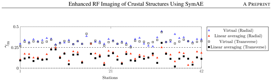
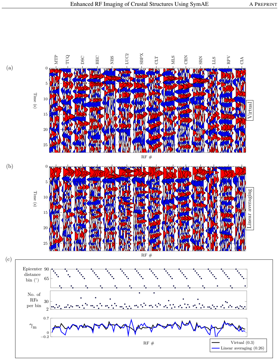
- [Appendix D.2, Eq. (D.2)] The real-data quality metric MNCC is computed between each virtual RF and the raw RFs in the same datapoint that was used to train the network and to accumulate the crustal posterior. This metric therefore measures self-consistency with the training distribution rather than fidelity to true crustal structure; a smooth virtual RF close to the average of noisy inputs can score highly without preserving genuine converted phases. The consistently higher MNCC of virtual RFs relative to linearly averaged RFs is thus not, on its own, evidence of enhanced crustal information in real data. An independent evaluation is needed, such as comparison with known interface depths, holdout stations or events, synthetic ground truth corrupted with real noise, or consistency checks against independent geophysical constraints.
- [Section 3.2, Eqs. (9)–(11)] The optimization that selects the optimal nuisance code uses the same encoder that defines Q(q|rj), so minimizing the KL divergence in Eq. (9) ensures that the virtual RF's crustal posterior matches the accumulated posterior, but it does not by itself guarantee that nuisance effects are minimized in any absolute sense. In addition, Eq. (11) reuses one optimal nuisance code for all datapoints of a station, which assumes that nuisance effects are transferable across backazimuth and epicentral distance; this assumption is not justified or tested. I suggest diagnostics such as repeating the virtual-RF generation with different nuisance-code initializations and reporting the spread of the resulting RFs, and comparing station-level results when the nuisance code is taken from a bin other than the highest-count bin.
- [Section 4] The synthetic setup states that the epicentral distance spans from 50° to 60° with 10°-interval bins, which yields one epicentral-distance bin, yet the text reports '36 × 6 × 6 synthetic datapoints'. The count should be 36 × 6 × 1, or else the number of epicentral-distance bins must be stated explicitly. This inconsistency affects the reproducibility of the training dataset description.
minor comments (7)
- [Section 3.1, Eq. (7)] The notation Q(q | rj, μq) appears after Eq. (7) and is inconsistent with the earlier notation Q(q | rj); the extra parameter μq is not defined and should be removed or clarified.
- [Figure 2] The caption text appears to mislabel the subplots: it says '(b) shows a reconstructed radial RF ... related to a station with a 27 km thick crust' while the figure panel labels and the surrounding text refer to different panel letters; the correspondence between panels (a)–(d) and the described crustal thicknesses should be corrected.
- [Section 3.2, Eq. (12)] The union expression contains a corrupted symbol ('station »') instead of the station index κ; this should be fixed.
- [Appendix D.2] The metric in Eq. (D.2) is written for yopt_j while the virtual RF in the main text is denoted yvirt_j in Eq. (10); the notation should be unified.
- [Appendix E.1] The statement that training was stopped at 190 epochs 'where the reconstruction loss of both the training and testing dataset converged' is vague; providing learning curves or a convergence criterion would improve reproducibility.
- [Section 4 / Figure 4] The phase-weighted averaging results are reported only for power ν = 0.8; a brief sensitivity statement for ν would clarify how the comparison depends on this choice.
- [Section 5.1] There are minor typographical spacing issues, such as 'V ancouver Island' and 'normalised' in Figure 13; these should be corrected in the final version.
Circularity Check
Real-data MNCC partly measures self-consistency with the datapoint RFs used to construct the virtual RF; the synthetic benchmark and geological comparisons provide independent, non-circular support.
-
fitted input called prediction
[Sec. 3.2 (Eqs. 7 and 10) vs. Appendix D.2 (Eq. D.2)]
"In real data applications, since there is no true RF, we calculate the mean normalized correlation coefficient (MNCC) of nuisance-minimized RF with the raw RFs in a datapoint. For instance, the MNCC of the optimized virtual RF yopt_j, related to the datapoint rj, is given by µm(yopt_j, rj) = 1/nj Σ_i µ(yopt_j, r_i_j)."
By Eq. 7, the accumulated crustal posterior Q(q|rj) is the product of per-RF posteriors Q(q|r_i_j), and qbar_j is its mean; by Eq. 10, yvirt_j = f(qbar_j, m_hat_virt). Thus the virtual RF is a deterministic function of every raw RF r_i_j in the datapoint. Eq. D.2 then averages the correlation of this same yvirt_j with those same r_i_j, so the reported MNCC is in part a self-consistency score with the datapoint RFs used to compute qbar_j, not an independent measure of crustal fidelity. The paper explicitly avoids this self-correlation for the linear-stack baseline in Eq. D.3 by excluding the compared RF from the average, making the real-data comparison statistically asymmetric and partly forced by construction.
full rationale
The core derivation of virtual RFs is not circular: the latent code qbar_j is an unsupervised summary of the datapoint, the decoder is trained with a standard ELBO, and the synthetic experiment scores virtual RFs against true noise-free RFs that were not used to build qbar_j. The Supplementary admission that deep converted phases are lost for thicker crust (Stations 4-6) is an honest correctness limitation, not circularity. The self-citations to Bharadwaj (2024) are not scored as load-bearing because the architecture and KL criterion are reimplemented in Appendix E and tested independently. However, the real-data MNCC evaluation is partially circular: Eq. D.2 correlates the virtual RF with the same datapoint RFs from which the accumulated code and the virtual RF were generated, while the linear-averaging baseline is evaluated leave-one-out (Eq. D.3). This asymmetry inflates the claimed real-data advantage, so the paper deserves a moderate circularity score despite its independent synthetic grounding.
Assumptions & free parameters
free parameters (3)
- Latent code lengths (q, p) =
q=50 (synthetic), 100 (real); p=20
- Backazimuth bin width =
10 deg (synthetic), 8 deg (real)
- Epicentral-distance bin width =
10 deg (synthetic), 5 deg (real)
assumptions (5)
- domain assumption Crustal effects are coherent across RFs within a backazimuth-slowness bin
- domain assumption Nuisance effects are RF-specific and can be represented by a low-dimensional latent code independent of the coherent code
- domain assumption RFs within a bin are independent observations
- ad hoc to paper A single optimal nuisance code can represent nuisance effects for all datapoints of a station
- standard math Standard normal prior on latent variables
Cite this review
Pith. "Pith review of Enhanced receiver function imaging of crustal structures using symmetric autoencoders." pith.science (2026). https://pith.science/paper/2RXZMQRJ
@misc{pith2026241114182,
  author       = {Pith},
  title        = {Pith review of: Enhanced receiver function imaging of crustal structures using symmetric autoencoders},
  year         = {2026},
  howpublished = {\url{https://pith.science/paper/2RXZMQRJ}},
  note         = {Machine review of arXiv:2411.14182}
}
read the original abstract
The receiver-function (RF) technique aims to recover receiver-side crustal and mantle structures by deconvolving either the radial or transverse component with the vertical component seismogram. Analysis of the variations of RFs along the backazimuth and slowness is the key in determining the geometry and anisotropic properties of the crustal structures. However, the deconvolution introduces pseudorandom nuisance effects, due to unknown earthquake source signatures and seismic noise, which obstruct the precise extraction of backazimuth and slowness dependent crustal effects. Our goal is to obtain RFs with minimal nuisance effects, while preserving the crustal effects. In this study, we introduced a new method for reducing nuisance effects in RFs. This method generates virtual RFs through a deep generative model, namely symmetric variational autoencoders (SymVAE). Our autoencoder efficiently learns to disentangle coherent crustal effects and nuisance effects within its latent space, given a set of RFs derived from a cluster of nearby earthquakes. This disentanglement enables generation of virtual RFs which exhibits minimal nuisance effects while preserving the coherent crustal effects. We tested SymVAE using synthetic RFs with ambient seismic noise. We also tested using dense seismic networks in two distinct geological settings: the Cascadia subduction zone and southern California. We compared our method with linear and phase-weighted averaging. In both synthetic and real RFs, the generated virtual RFs demonstrate enhanced information related to crustal structures. We have also quantitatively assessed the performance. One major advantage of our method over traditional methods is its ability to utilize all available earthquake data, regardless of signal quality, resulting in improved backazimuth and slowness coverage.
Figures


Figures from the paper (19 more)






Reference graph
Works this paper leans on
-
[1]
Seismic anisotropy indicators in western tibet: Shear wave splitting and receiver function analysis
Vadim Levin, Steven Roecker, Peter Graham, and Ali Hosseini. Seismic anisotropy indicators in western tibet: Shear wave splitting and receiver function analysis. Tectonophysics, 462 0 (1): 0 99--108, 2008. doi:10.1016/j.tecto.2008.03.019
-
[2]
Augmented fidelities for single qubit gates
Martha K. Savage, J. Park, and H. Todd. Velocity and anisotropy structure at the hikurangi subduction margin, new zealand from receiver functions. Geophysical Journal International, 168 0 (3): 0 1034--1050, March 2007. doi:10.1111/j.1365-246X.2006.03086.x
work page Pith review arXiv 2007
-
[3]
Zhen Liu, Jeffrey Park, and Danny M Rye. Crustal anisotropy in northeastern tibetan plateau inferred from receiver functions: Rock textures caused by metamorphic fluids and lower crust flow? Tectonophysics, 661: 0 66--80, 2015. doi:10.1016/j.tecto.2015.08.006
-
[4]
D. E. McNamara and T. J. Owens. Azimuthal shear‐wave velocity anisotropy in the basin and range province using moho ps converted phases. Journal of Geophysical Research, 98 0 (B7): 0 12003--12017, 1993. doi:10.1029/93JB00711
-
[5]
I. Bianchi, J. Park, N. Piana Agostinetti, and V. Levin. Mapping seismic anisotropy using harmonic decomposition of receiver functions: An application to northern apennines, italy. Journal of Geophysical Research, 115: 0 B12317, 2010. doi:10.1029/2009JB007061
-
[6]
T. Zheng, Z. Ding, J. Ning, L. Chang, X. Wang, and F. et al. Kong. Crustal azimuthal anisotropy beneath the southeastern tibetan plateau and its geodynamic implications. Journal of Geophysical Research: Solid Earth, 123: 0 9733--9749, 2018. doi:10.1029/2018JB015995
-
[7]
Katsuhiko Shiomi and Jeffrey Park. Structural features of the subducting slab beneath the kii peninsula, central japan: Seismic evidence of slab segmentation, dehydration, and anisotropy. Journal of Geophysical Research: Solid Earth, 113 0 (B10), 2008. doi:https://doi.org/10.1029/2007JB005535. URL https://agupubs.onlinelibrary.wiley.com/doi/abs/10.1029/20...
-
[8]
Moho depth variation in southern california from teleseismic receiver functions
Lupei Zhu and Hiroo Kanamori. Moho depth variation in southern california from teleseismic receiver functions. Journal of Geophysical Research: Solid Earth, 105 0 (B2): 0 2969--2980, 2000
work page 2000
Show all 65 references
-
[9]
Kolb and V
J. Kolb and V. Lekić. Receiver function deconvolution using transdimensional hierarchical bayesian inference. Geophysical Journal International, 197 0 (3): 0 1719--1735, 2014
2014
-
[10]
Inversion of receiver functions without deconvolution—application to the indian craton
Thomas Bodin, Huaiyu Yuan, and Barbara Romanowicz. Inversion of receiver functions without deconvolution—application to the indian craton. Geophysical Journal International, 196 0 (2): 0 1025–1033, February 2014. doi:10.1093/gji/ggt431
2014 doi
-
[11]
Variance estimate in frequency-domain deconvolution for teleseismic receiver function computation
Massimo Bona. Variance estimate in frequency-domain deconvolution for teleseismic receiver function computation. Geophysical Journal International, 134 0 (2): 0 634--646, 1998. doi:10.1111/j.1365-246X.1998.tb07128.x
1998 doi
-
[12]
Akuhara, M
T. Akuhara, M. G. Bostock, A. P. Plourde, and M. Shinohara. Beyond receiver functions: Green's function estimation by transdimensional inversion and its application to obs data. Journal of Geophysical Research: Solid Earth, 124 0 (2): 0 1944--1961, 2019. doi:10.1029/2018JB016499
1944 doi
-
[13]
Park and V
J. Park and V. Levin. Receiver functions from multiple‐taper spectral correlation estimates. Bull. Seism. Soc. Am., 90 0 (6): 0 1507--1520, 2000
2000
-
[14]
Zhang, Y
Q. Zhang, Y. Chen, F. Zhang, and Y. Chen. Improving receiver function imaging with high-resolution radon transform. Geophysical Journal International, 230 0 (2): 0 1292–1304, March 2022. doi:10.1093/gji/ggac116
2022 doi
-
[15]
Crustal imaging with noisy teleseismic receiver functions using sparse radon transforms
Ziqi Zhang and Tolulope Olugboji. Crustal imaging with noisy teleseismic receiver functions using sparse radon transforms. Bulletin of the Seismological Society of America, 114 0 (3): 0 1600--1612, 2024. doi:10.1785/0120230254
2024 doi
-
[16]
H. P. Crotwell and T. J. Owens. Automated receiver function processing. Seismological Research Letters, 76 0 (6): 0 702--709, 2005. doi:10.1785/gssrl.76.6.702
2005 doi
-
[17]
Pavlis, and Yibo Wang
Xiaoning Yang, Gary L. Pavlis, and Yibo Wang. A quality control method for teleseismic p-wave receiver functions. Bulletin of the Seismological Society of America, 106 0 (5): 0 1948--1962, 2016. doi:10.1785/0120150347
1948 doi
-
[18]
C. Gong, L. Chen, Z. Xiao, and X. Wang. Deep learning for quality control of receiver functions. Frontiers in Earth Science, 2022. doi:10.3389/feart.2022.921830
2022
-
[19]
H. E. Krueger, I. Gama, and K. M. Fischer. Global patterns in cratonic mid-lithospheric discontinuities from sp receiver functions. Geochemistry, Geophysics, Geosystems, 22 0 (6), 2021. doi:10.1029/2021GC009819
2021 doi
-
[20]
Sabermahani and A
S. Sabermahani and A. Frederiksen. Deeprfqc: automating quality control for p-wave receiver function analysis using a u-net inspired network. Seismica, 3 0 (2), 2024. doi:10.26443/seismica.v3i2.1341
2024 doi
-
[21]
Gurrola, G
H. Gurrola, G. E. Baker, and J. B. Minster. Simultaneous time domain deconvolution with application to the computation of receiver functions. Geophys. J. Int., 120: 0 537--543, 1995
1995
-
[22]
Levin and J
V. Levin and J. Park. Crustal anisotropy beneath the ural mtns foredeep from teleseismic receiver functions. Geophys. Res. Lett., 24: 0 1283--1286, 1997
1997
-
[23]
A review on the analysis of the crustal and upper mantle structure using receiver functions
Jiafu Hu, Haiyan Yang, Guangquan Li, and Hengchu Peng. A review on the analysis of the crustal and upper mantle structure using receiver functions. Journal of Asian Earth Sciences, 111: 0 589--603, 2015. ISSN 1367-9120. doi:10.1016/j.jseaes.2015.06.007
2015 doi
-
[24]
Bloch, M
W. Bloch, M. G. Bostock, and P. Audet. A cascadia slab model from receiver functions. Geochemistry, Geophysics, Geosystems, 24 0 (10): 0 e2023GC011088, 2023. doi:10.1029/2023GC011088
2023 doi
-
[25]
Schimmel and H
M. Schimmel and H. Paulssen. Noise reduction and detection of weak, coherent signals through phase-weighted stacks. Geophysical Journal International, 130: 0 497--505, 1997
1997
-
[26]
Ozakin and Y
Y. Ozakin and Y. Ben-Zion. Systematic receiver function analysis of the moho geometry in the southern california plate-boundary region. Pure and Applied Geophysics, 172: 0 1167--1184, 2015. doi:10.1007/s00024-014-0924-6
2015 doi
-
[27]
Olugboji, Z
T. Olugboji, Z. Zhang, S. Carr, C. Ekmekci, and M. Cetin. On the detection of upper mantle discontinuities with radon-transformed ps receiver functions (crisp-rf), June 2023
2023
-
[28]
Denoising the receiver function through curvelet transforming and migration imaging
Yan Chen, Jian Chen, Bengang Guo, Shuyun Qi, and Ping Zhao. Denoising the receiver function through curvelet transforming and migration imaging. Chinese Journal of Geophysics, 62 0 (6): 0 2027--2037, 2019
2027
-
[29]
R. M. H. Dokht, Y. J. Gu, and M. D. Sacchi. Singular spectrum analysis and its applications in mapping mantle seismic structure. Geophysical Journal International, 208 0 (3): 0 1430--1442, December 2016. doi:10.1093/gji/ggw473
2016 doi
-
[30]
F. Wang, X. Song, and J. Li. Deep learning-based h- method (hknet) for estimating crustal thickness and vp/vs ratio from receiver functions. Journal of Geophysical Research: Solid Earth, 127 0 (6), June 2022. doi:10.1029/2022jb023944
2022 doi
-
[31]
L. Zhu. Crustal structure across the san andreas fault, southern california from teleseismic converted waves. Earth planet. Sci. Lett., 179: 0 183--190, 2000
2000
-
[32]
Seismic imaging of crustal reworking and lithospheric modification in eastern china
Tian-Yu Zheng, Liang Zhao, Yu-Mei He, and Ri-Xiang Zhu. Seismic imaging of crustal reworking and lithospheric modification in eastern china. Geophysical Journal International, 196 0 (2): 0 656--670, February 2014. doi:10.1093/gji/ggt420
2014 doi
-
[33]
Kingma and Max Welling
Diederik P. Kingma and Max Welling. Auto-encoding variational bayes. In ICLR, 2014
2014
-
[34]
Denoising diffusion probabilistic models, 2020
Jonathan Ho, Ajay Jain, and Pieter Abbeel. Denoising diffusion probabilistic models, 2020. URL https://arxiv.org/abs/2006.11239
2020 arXiv
-
[35]
Prince, and Marcus A
Ivan Kobyzev, Simon J.D. Prince, and Marcus A. Brubaker. Normalizing flows: An introduction and review of current methods. IEEE Transactions on Pattern Analysis and Machine Intelligence, 43 0 (11): 0 3964–3979, November 2021. ISSN 1939-3539. doi:10.1109/tpami.2020.2992934. URL...
2021
-
[36]
Christopher M. Bishop. Deep Learning. Springer, New York, NY, 2023. ISBN 978-3-030-12345-6
2023
-
[37]
Valentine and Jeannot Trampert
Andrew P. Valentine and Jeannot Trampert. Data space reduction, quality assessment and searching of seismograms: autoencoder networks for waveform data. Geophysical Journal International, 189 0 (2): 0 1183--1202, May 2012. doi:10.1111/j.1365-246X.2012.05429.x
2012 arXiv
-
[38]
Ning and Y
C. Ning and Y. Xie. Convolutional variational autoencoder for ground motion classification and generation toward efficient seismic fragility assessment. Computer-Aided Civil and Infrastructure Engineering, 39: 0 165--185, 2024. doi:10.1111/mice.13061
2024 doi
-
[39]
Fayaz and C
J. Fayaz and C. Galasso. A deep neural network framework for real-time on site estimation of acceleration response spectra of seismic ground motions. Computer-Aided Civil and Infrastructure Engineering, 38: 0 87--103, 2023. doi:10.1111/mice.12830
2023 doi
-
[40]
Disentangling factors of variation in deep representation using adversarial training
Michael F Mathieu, Junbo Jake Zhao, Junbo Zhao, Aditya Ramesh, Pablo Sprechmann, and Yann LeCun. Disentangling factors of variation in deep representation using adversarial training. Advances in Neural Information Processing Systems, 29, 2016. URL https://proceedings.neurips.c...
2016
-
[41]
Burgess, Irina Higgins, Arka Pal, Loic Matthey, Nick Watters, Guillaume Desjardins, and Alexander Lerchner
Christopher P. Burgess, Irina Higgins, Arka Pal, Loic Matthey, Nick Watters, Guillaume Desjardins, and Alexander Lerchner. Understanding disentangling in -vae, 2018. URL https://arxiv.org/abs/1804.03599
2018 arXiv
-
[42]
On extracting coherent seismic wavefield using variational symmetric autoencoders, 2024
Pawan Bharadwaj. On extracting coherent seismic wavefield using variational symmetric autoencoders, 2024. URL https://arxiv.org/abs/2411.15613
2024 arXiv
-
[43]
Receiver functions from seismic interferometry: a practical guide
Benoit Tauzin, Thanh-Son Pham, and Hrvoje Tkalčić. Receiver functions from seismic interferometry: a practical guide. Geophysical Journal International, 217 0 (1): 0 1--24, April 2019. doi:10.1093/gji/ggz002
2019 doi
-
[44]
Simon J. D. Prince. Understanding Deep Learning. The MIT Press, 2023. ISBN 9780262048644
2023
-
[45]
Inverse problem theory and methods for model parameter estimation
Albert Tarantola. Inverse problem theory and methods for model parameter estimation. SIAM, 2005
2005
-
[46]
Pyraysum: Software for modeling ray-theoretical plane body-wave propagation in dipping anisotropic media
Wasja Bloch and Pascal Audet. Pyraysum: Software for modeling ray-theoretical plane body-wave propagation in dipping anisotropic media. Seismica, 2 0 (1), Feb. 2023. doi:10.26443/seismica.v2i1.220. URL https://seismica.library.mcgill.ca/article/view/220
2023 doi
-
[47]
Portable observatories for lithospheric analysis and research investigating seismicity, 2000
Geological Survey of Canada . Portable observatories for lithospheric analysis and research investigating seismicity, 2000. URL https://www.fdsn.org/networks/detail/PO/
2000
-
[48]
Canadian seismic research network, 2002
Geological Survey of Canada . Canadian seismic research network, 2002. URL https://www.fdsn.org/networks/detail/C8/
2002
-
[49]
Canadian national seismograph network, 1975
Natural Resources Canada . Canadian national seismograph network, 1975. URL https://www.fdsn.org/networks/detail/CN/
1975
-
[50]
Pacific northwest seismic network - university of washington, 1963
University of Washington . Pacific northwest seismic network - university of washington, 1963. URL https://www.fdsn.org/networks/detail/UW/
1963
-
[51]
California institute of technology, caltech, 1926
SCSN. California institute of technology, caltech, 1926. Other/Seismic Network
1926
-
[52]
J.F. Cassidy. A comparison of the receiver structure beneath stations of the canadian national seismograph network. Canadian Journal of Earth Sciences, 32: 0 938--951, 1995
1995
-
[53]
C. A. Langston. Structure under mount rainier, washington, inferred from teleseismic body waves. J. Geophys. Res., 84: 0 4749--4762, 1979
1979
-
[54]
Nicholson, M
T. Nicholson, M. Bostock, and J. F. Cassidy. New constraints on subduction zone structure in northern cascadia. Geophysical Journal International, 161 0 (3): 0 849--859, June 2005. doi:10.1111/j.1365-246X.2005.02605.x
2005 arXiv
-
[55]
Bostock, Norman I
Pascal Audet, Michael G. Bostock, Norman I. Christensen, and Sheila M. Peacock. Seismic evidence for overpressured subducted oceanic crust and megathrust fault sealing. Nature, 457 0 (7225): 0 76–78, 2009. doi:10.1038/nature07650
2009 doi
-
[56]
DeMets, R
C. DeMets, R. G. Gordon, D. F. Argus, and S. Stein. Effect of recent revisions to the geomagnetic reversal time scale on estimates of current plate motions. Geophysical Research Letters, 21 0 (20): 0 2191--2194, 1994. doi:10.1029/94gl02118
1994 doi
-
[57]
Crustal geophysics and seismicity in southern california
Egill Hauksson. Crustal geophysics and seismicity in southern california. Geophysical Journal International, 186 0 (1): 0 82--98, July 2011. doi:10.1111/j.1365-246X.2011.05042.x
2011 arXiv
-
[58]
Shaw, Andreas Plesch, Carl Tape, M
John H. Shaw, Andreas Plesch, Carl Tape, M. Peter Suess, Thomas H. Jordan, Geoffrey Ely, Egill Hauksson, Jeroen Tromp, Toshiro Tanimoto, Robert Graves, Kim Olsen, Craig Nicholson, Philip J. Maechling, Carlos Rivero, Peter Lovely, Charles M. Brankman, and Jason Munster. Unified...
2015 doi
-
[59]
Refined crustal and uppermost mantle structure of southern california by ambient noise adjoint tomography
Kai Wang, Yingjie Yang, Piero Basini, Ping Tong, Carl Tape, and Qinya Liu. Refined crustal and uppermost mantle structure of southern california by ambient noise adjoint tomography. Geophysical Journal International, 215 0 (2): 0 844--863, November 2018. doi:10.1093/gji/ggy312
2018 doi
-
[60]
Arda Ozacar and George Zandt
A. Arda Ozacar and George Zandt. Crustal structure and seismic anisotropy near the san andreas fault at parkfield, california. Geophysical Journal International, 178 0 (2): 0 1098--1104, August 2009. doi:10.1111/j.1365-246X.2009.04198.x
2009 arXiv
-
[61]
P. Wang, Z. Huang, and X. Wang. A method for estimating the crustal azimuthal anisotropy and moho orientation simultaneously using receiver functions. Journal of Geophysical Research: Solid Earth, 125: 0 e2019JB018405, 2020. doi:10.1029/2019JB018405
2020 doi
-
[62]
Fashionable modelling with flux
Michael Innes, Elliot Saba, Keno Fischer, Dhairya Gandhi, Marco Concetto Rudilosso, Neethu Mariya Joy, Tejan Karmali, Avik Pal, and Viral Shah. Fashionable modelling with flux. CoRR, abs/1811.01457, 2018. URL https://arxiv.org/abs/1811.01457
2018 arXiv
-
[63]
Hosseini and K
K. Hosseini and K. Sigloch. Obspydmt: a python toolbox for retrieving and processing large seismological data sets. Solid Earth, 8: 0 1047--1070, 2017. doi:10.5194/se-8-1047-2017
2017 doi
-
[64]
Source shape estimation and deconvolution of teleseismic body waves
Robert W Clayton and Robert A Wiggins. Source shape estimation and deconvolution of teleseismic body waves. J. R. Astr. Soc., 47: 0 151--177, 1976
1976
-
[65]
Imagenet classification with deep convolutional neural networks
Alex Krizhevsky, Ilya Sutskever, and Geoffrey E Hinton. Imagenet classification with deep convolutional neural networks. In Advances in Neural Information Processing Systems, volume 25. Curran Associates, Inc., 2012
2012
Reviewed August 12, 2026 · model on record in the stance chip above.
Discussion (0). Continue with ORCID to comment.