REVIEW 4 major objections 4 minor 29 references
Quantum-Enhanced Spectral Solution of the Poisson Equation
T0 review · 4 major / 4 minor · reviewed 2026-08-07 · deepseek-v4-flash
Pith's one-line read A hybrid quantum-classical method estimates Poisson solution coefficients by measuring the Quantum Fourier Transform of the source and dividing by Laplacian eigenvalues.
desk verdict The accuracy comes from fitted per-source corrections, not from the QFT; the central claim of a general quantum spectral solver does not hold up, though the paper is a clear and honest benchmark of overhead. read the letter →
The pith
A machine-rendered reading of the paper's core claim, the machinery that carries it, and where it could break.
The reading
What carries the argument
The central object is the two-dimensional Quantum Fourier Transform, the quantum analogue of the discrete Fourier transform, applied to the discretized and normalized source state $|\psi\rangle$. After the transform, each basis state $|k,l\rangle$ is measured with probability $P(k,l)=|\tilde\psi_{kl}|^2$, so the magnitudes of the spectral coefficients are estimated as $\sqrt{C_{kl}/S}$ from shot counts $C_{kl}$ and total shots $S$. These magnitudes are turned into signed coefficients by a correction factor, then divided by the Laplacian eigenvalue $\lambda_{ij}=((i+1)\pi/L_x)^2+((j+1)\pi/L_y)^2$, and the solution is the sine-series sum of those quotients. The QFT is what converts an $O(2^{n+m})$ double-sum integration into an $O(n^2+m^2)$ circuit.
What would settle it
Run the method on a source not covered by the four test families, for example $f(x,y)=\sin(2\pi x)\sin(\pi y)+\sin(\pi x)\sin(3\pi y)$, using the correction formula in Eq. (20); if the reconstructed solution's mean squared error degrades by more than an order of magnitude relative to the reported $10^{-6}$ to $10^{-10}$ range, the correction is source-specific and the general claim fails.
Extended reading notes
Core claim
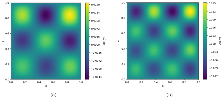
The central discovery is that the QFT measurement probabilities of the normalized source state already contain the spectral information needed to solve the Poisson equation, so the integration-heavy coefficient step can be replaced by counting measurement outcomes. The reconstructed solution is $u(x,y)=\sum_{i,j} \mathrm{Re}(a_{ij})/\lambda_{ij}\,\phi_{ij}(x,y)$, where $a_{ij}$ are the normalized square-root-count amplitudes and $\lambda_{ij}$ are the eigenvalues of the Laplacian. A per-source phase and spectral correction is applied to recover the sign information that squared magnitudes lose. The paper's numerical experiments show that this reconstruction matches the classical spectral solution to high accuracy across several families of source functions, and its benchmarks show that the quantum coefficient step is substantially cheaper in time and slightly cheaper in memory.
Load-bearing premise
The load-bearing premise is that the magnitudes of QFT measurement counts, plus the paper's fixed phase and spectral correction formulas, uniquely determine the signed sine-series coefficients for any source function.
Editorial extensions
If this is right
- For large grids, the coefficient-estimation step stops being the computational bottleneck: the QFT circuit costs $O(n^2+m^2)$ instead of the $O(2^{n+m})$ double-sum or the FFT's $O(2^n\log 2^n)$ cost, and the benchmark shows a 93.9% reduction in that phase.
- The classical solution-reconstruction step, not the quantum part, becomes the dominant cost, so truncating the sine series during reconstruction directly controls the remaining runtime.
- If the measured magnitudes are accurate enough, the same eigenvalue-division scheme applies to other separable elliptic problems with known eigenfunctions, not only the rectangular Poisson case.
- The reported memory footprint is about 14% lower overall on a 256 by 256 grid, with the largest saving in coefficient processing.
- The accuracy and complexity results together suggest that the method is most attractive when the number of grid points is large enough that classical integration becomes prohibitive.
Reading between the lines
- Because the method reads only magnitudes of the transformed amplitudes, the sign and phase recovery is a phase-retrieval problem in disguise; the per-source correction formulas suggest that a generic phase-recovery step would be needed before the method can be applied to arbitrary right-hand sides.
- A natural next test is to replace the shot-count estimate $\sqrt{C_{kl}/S}$ with a quantum amplitude estimation procedure, which would reduce sampling noise at similar circuit depth and likely lower the achievable mean squared error.
- The efficiency comparison uses simulated, effectively noiseless circuits; on real hardware, state preparation and measurement errors would add overhead that the current benchmarks do not price in.
- The reported speedup is specific to the coefficient phase, and any total-speedup claim depends on amortizing state preparation, which the paper shows grows with qubit count.
Editorial analysis
A structured set of objections, weighed in public.
Referee Report
Summary. The manuscript proposes a hybrid quantum-classical spectral solver for the 2D Poisson equation with homogeneous Dirichlet boundary conditions. The source is normalized and encoded into a quantum state, a 2D QFT is applied, measurement counts are used to estimate magnitudes of Fourier coefficients, and the solution is reconstructed from sine modes divided by Laplacian eigenvalues. Numerical experiments on sinusoidal, anisotropic polynomial, Gaussian, and combined sources report MSEs between 3.20e-10 and 2.91e-6, and Section 4 claims large reductions in time and memory compared with a classical implementation. The paper concludes that the approach is a promising starting point for quantum-assisted PDE solvers.
Significance. Taken at face value, a general method that obtains spectral coefficients of the Poisson solution directly from QFT measurements with polylogarithmic complexity would be a significant result for quantum numerical analysis. The manuscript, however, does not establish such a general method: the link between measured probabilities and signed coefficients is completed by per-source correction factors (Eqs. 20, 22, 24, 26) that are fitted experimentally. The main contribution is therefore a set of benchmark-specific reconstructions, not a validated algorithm for arbitrary source terms. The paper is transparent about its simulated setting and about the need for classical correction and HPC interoperability, which is commendable, but those admissions underscore the missing theoretical core. No code or machine-checked proofs are provided.
major comments (4)
- [Sec. 2.2, Eqs. (10)-(12); Sec. 3, Eqs. (20),(22),(24),(26)] The quantum measurement yields only probabilities P(k,l)=|ψ̃_kl|^2, from which only magnitudes |ψ̃_kl| are recovered. The signs and relative phases of the sine-series coefficients are not obtainable from these data. The paper compensates by multiplying the magnitudes by source-specific correction factors—e.g., exp(-iπ(m+n)/2)·(mn)^2/(m+n)^3 for sinusoidal sources, exp(-iπ(m+n))·(mn)^2/(m+n)^3 for the anisotropic polynomial, exp(-iπ mn/2) for the Gaussian, and exp(-iπ mn)·(mn)^2/(m^2+n^2)^{3/2} for the sum—described as "determined experimentally" with no derivation from the QFT or from the Poisson equation. Consequently the reported MSEs demonstrate that the coefficients can be fitted for the tested functions; they do not validate the claim that the method estimates coefficients for an arbitrary source f. Since the abstract and conclusions assert a general quantum-enhanced spectral method, this is the central load-bearing defect.
- [Sec. 3, Eq. (19)] The "shifting procedure" k1 = m1 + shift(m1), with shift(m)=0 for m≤2 and shift(m)=m−2 otherwise, changes the actual source function for every m>2. The paper provides no justification for this shift beyond "to ensure correct harmonic retrieval," so the sinusoidal benchmarks do not correspond to a fixed family of sources under a single algorithm; the shift is another source-specific adjustment. A general method should either include a principled rule for choosing its parameters or state clearly that the algorithm requires per-problem calibration.
- [Sec. 4.1-4.2, Table 1, Table 2, Figures 11-13] The complexity comparison is not made against the relevant classical baseline. Table 1 lists the FFT complexity O(2^n log 2^n + 2^m log 2^m), but the benchmarks in Table 2 and Figures 11-13 use a classical implementation based on "numerical approximation of the integral" (dblquad), which is the O(2^{n+m}) direct method quoted as inefficient. Comparing QFT time against dblquad time therefore inflates the reported 93.9% coefficient-calculation speedup. In addition, the quantum timing includes state preparation (3.34 s) but does not report the number of measurement shots, the QFT simulation overhead, or the cost of the correction step in all runs; without these, the claimed end-to-end speedup is not established.
- [Eq. (18) and Sec. 3] The reconstruction formula u(x,y)=Σ Re(a_ij)/λ_ij φ_ij uses Re(a_ij), but at that point a_ij denotes the positive magnitudes from Eq. (13); the corrected complex coefficients B_mn are never explicitly substituted into Eq. (18). This makes it unclear whether the plotted solutions are reconstructed from Re(B_mn), |B_mn|, or some other combination, and prevents the reader from reproducing the MSEs. This is a clarity issue, but in combination with the fitted corrections it obscures what the numerical experiments actually validate.
minor comments (4)
- [Eqs. (2)-(4), Eq. (17)] The indexing is inconsistent: Eq. (3) uses sin((k_x+1)πx/L_x), while Eq. (4) uses sin(k_x πx/L_x); Eq. (2) defines φ_{k_x k_y} without the +1, while Eq. (17) includes it. Please harmonize the notation.
- [Table 1] The entry "Quasi linear" is inaccurate: O(n^2+m^2) is polynomial in the number of qubits and polylogarithmic in the grid dimension, not quasi-linear in the usual O(N log N) sense.
- [Sec. 3] The paper does not report the number of shots used in the measurements or the qubit counts and truncation parameters (τ_x,τ_y) for each experiment, which are needed to assess the MSE values and the truncation claims in Figure 6.
- [Sec. 3] There are several typos and stylistic issues, e.g., ",,so" in Section 3 and the inconsistent use of "anisotropic"/"anisotropy"; a careful proofread is needed.
Circularity Check
Measured probabilities supply only |a_kl|; the reconstruction uses signed Re(a_kl) with source-specific fitted phase/spectral corrections (Eqs. 20–26), so the claimed coefficient prediction reduces to per-benchmark fits.
-
fitted input called prediction
[Section 2.2, Eqs. (10)–(18)]
"P(k, l) = |ψ̃_kl|² ... The magnitude of the frequencies amplitude is approximated by |ψ̃_kl| ≈ sqrt(C_kl/S) ... Since the coefficients a_ij can be complex due to the quantum state, we take their real part in the final reconstruction. u(x,y)=Σ Re(a_ij)/λ_ij φ_ij(x,y)."
The QFT measurement determines only the modulus-squared of transformed amplitudes. Eq. (18) nevertheless reconstructs the solution from signed Re(a_ij). No equation in the paper derives sign or phase information from the counts C_kl; the transition from |ψ̃_kl| to Re(a_ij) is not a derivation. All sign and relative-phase information has to be supplied externally by the per-case correction factors in Eqs. (20)–(26). Thus the coefficients are not estimated directly within the quantum framework; their signs are injected classically.
-
fitted input called prediction
[Section 3, Eqs. (20), (22), (24), (26)]
"After obtaining the coefficients from Eq.(13), a correction was applied to address the loss of relative phase information after the measurements... Bmn = amn · exp(−iπ(m+n)/2) · (mn)²/(m+n)³ ... In this case, the optimal phase factor determined experimentally was found to be: Bmn = amn · exp(−iπmn/2) ... Bmn = amn · exp(−iπmn) (mn)²/(m²+n²)^{3/2}."
Each benchmark source is given its own phase factor and spectral rescaling, and for the Gaussian and sum cases the factor is explicitly determined experimentally. The factors are not derived from the QFT or from Δu=f, and they differ from one test to the next (Eq. 20 vs. Eq. 22 vs. Eq. 24 vs. Eq. 26). Multiplying the measured magnitude by a fitted phase and a fitted mode-dependent weight makes the final Bmn agree with the known classical coefficients for that particular f by construction. The reported MSEs therefore validate the fit for the benchmarked functions, not a transferable rule for arbitrary source functions.
full rationale
The paper does not rely on self-citations, and the spectral identity a_ij/λ_ij (Eq. 16) is the standard, non-circular Poisson-series relation. The circularity is located in the coefficient-estimation pipeline: the QFT measurement yields only probabilities P(k,l)=|ψ̃_kl|², so only magnitudes of the transformed amplitudes are accessible. The reconstructed solution (Eq. 18) requires signed Re(a_ij), and the missing signs and phases are installed through the source-dependent correction formulas in Eqs. (20), (22), (24), and (26), the last two of which are explicitly labeled as optimal phase factor determined experimentally. Because these corrections are fitted per benchmark function and differ between source classes, the claimed general method of estimating coefficients directly within the quantum framework reduces, for each demonstrated case, to fitting the classical solution. The complexity comparison in Section 4 also omits amplitude-encoding and shot-overhead costs, but that omission is a completeness issue rather than the central circularity. The central claim is partially circular: the reported accuracy is real for the fitted benchmarks, but it does not establish prediction for a new source. Score: 7.
Assumptions & free parameters
free parameters (6)
- shift function shift(m) in Eq. (19) =
0 if m <= 2 else m - 2
- Phase correction for sinusoidal sources Eq. (20) =
exp(-i*pi*(m+n)/2)
- Spectral correction for sinusoidal sources Eq. (20) =
(mn)^2/(m+n)^3
- Phase correction for anisotropic polynomial source Eq. (22) =
exp(-i*pi*(m+n))
- Phase correction for Gaussian source Eq. (24) =
exp(-i*pi*m*n/2)
- Correction for Gaussian+sin source Eq. (26) =
exp(-i*pi*m*n) * (mn)^2/(m^2+n^2)^(3/2)
assumptions (4)
- standard math Standard sine-series expansion of the Dirichlet Poisson solution
- domain assumption Arbitrary source f can be amplitude-encoded efficiently
- domain assumption Measurement statistics from finite shots give reliable coefficient magnitudes
- ad hoc to paper QFT sampled magnitudes correspond to sine coefficients after correction
Cite this review
Pith. "Pith review of Quantum-Enhanced Spectral Solution of the Poisson Equation." pith.science (2026). https://pith.science/paper/2SY7A7VE
@misc{pith2026250607743,
  author       = {Pith},
  title        = {Pith review of: Quantum-Enhanced Spectral Solution of the Poisson Equation},
  year         = {2026},
  howpublished = {\url{https://pith.science/paper/2SY7A7VE}},
  note         = {Machine review of arXiv:2506.07743}
}
read the original abstract
We present a hybrid numerical-quantum method for solving the Poisson equation under homogeneous Dirichlet boundary conditions, leveraging the Quantum Fourier Transform (QFT) to enhance computational efficiency and reduce time and space complexity. This approach bypasses the integration-heavy calculations of classical methods, which have to deal with high computational costs for large number of points. The proposed method estimates the coefficients of the series expansion of the solution directly within the quantum framework. Numerical experiments validate its effectiveness and reveal significant improvements in terms of time and space complexity and solution accuracy, demonstrating the capability of quantum-assisted techniques to contribute in solving partial differential equations (PDEs). Despite the inherent challenges of quantum implementation, the present work serves as a starting point for future researches aimed at refining and expanding quantum numerical methods.
Figures


Figures from the paper (11 more)


Reference graph
Works this paper leans on
-
[1]
What is the fast fourier transform? Proceedings of the IEEE, 55 0 (10): 0 1664--1674, 1967
William T Cochran, James W Cooley, David L Favin, Howard D Helms, Reginald A Kaenel, William W Lang, George C Maling, David E Nelson, Charles M Rader, and Peter D Welch. What is the fast fourier transform? Proceedings of the IEEE, 55 0 (10): 0 1664--1674, 1967
work page 1967
-
[2]
Practical quantum advantage in quantum simulation
Andrew J Daley, Immanuel Bloch, Christian Kokail, Stuart Flannigan, Natalie Pearson, Matthias Troyer, and Peter Zoller. Practical quantum advantage in quantum simulation. Nature, 607 0 (7920): 0 667--676, 2022
work page 2022
-
[3]
Methods of numerical integration
Philip J Davis and Philip Rabinowitz. Methods of numerical integration. Courier Corporation, 2007
work page 2007
-
[4]
Hybrid quantum-classical algorithms and quantum error mitigation
Suguru Endo, Zhenyu Cai, Simon C Benjamin, and Xiao Yuan. Hybrid quantum-classical algorithms and quantum error mitigation. Journal of the Physical Society of Japan, 90 0 (3): 0 032001, 2021
work page 2021
-
[5]
Lawrence C. Evans. Partial differential equations. American Mathematical Society, Providence, R.I., 2010. ISBN 9780821849743 0821849743
work page 2010
-
[6]
Jennifer Faj, Ivy Peng, Jacob Wahlgren, and Stefano Markidis. Quantum computer simulations at warp speed: Assessing the impact of gpu acceleration: A case study with ibm qiskit aer, nvidia thrust & cuquantum. In 2023 IEEE 19th International Conference on e-Science (e-Science), pages 1--10. IEEE, 2023
work page 2023
-
[7]
Hongsong Feng and Shan Zhao. Fft-based high order central difference schemes for three-dimensional poisson's equation with various types of boundary conditions. Journal of Computational Physics, 410: 0 109391, 2020
work page 2020
-
[8]
Rudolf J Freund and William J Wilson. Statistical methods. Elsevier, 2003
work page 2003
Show all 29 references
-
[9]
Numerical analysis
Walter Gautschi. Numerical analysis. Springer Science & Business Media, 2011
2011
-
[10]
Numerical analysis of spectral methods: theory and applications
David Gottlieb and Steven A Orszag. Numerical analysis of spectral methods: theory and applications. SIAM, 1977
1977
-
[11]
Wood, Jake Lishman, Julien Gacon, Simon Martiel, Paul D
Ali Javadi-Abhari, Matthew Treinish, Kevin Krsulich, Christopher J. Wood, Jake Lishman, Julien Gacon, Simon Martiel, Paul D. Nation, Lev S. Bishop, Andrew W. Cross, Blake R. Johnson, and Jay M. Gambetta. Quantum computing with qiskit, 2024. URL https://arxiv.org/abs/2405.08810
2024 arXiv
-
[12]
A new method based on the laplace transform and fourier series for solving linear neutral delay differential equations
Gilbert Kerr, Gilberto Gonzalez-Parra, and Michelle Sherman. A new method based on the laplace transform and fourier series for solving linear neutral delay differential equations. Applied Mathematics and Computation, 420: 0 126914, 05 2022. doi:10.1016/j.amc.2021.126914
2022
-
[13]
Classical and quantum computation
Alexei Yu Kitaev, Alexander Shen, and Mikhail N Vyalyi. Classical and quantum computation. Number 47. American Mathematical Soc., 2002
2002
-
[14]
Computational integration
Arnold R Krommer and Christoph W Ueberhuber. Computational integration. SIAM, 1998
1998
-
[15]
Hybrid quantum computing
Seth Lloyd. Hybrid quantum computing. In Quantum information with continuous variables, pages 37--45. Springer, 2003
2003
-
[16]
D. R. Musk. A comparison of quantum and traditional fourier transform computations. Computing in Science & Engineering, 22 0 (6): 0 103--110, 2020. doi:10.1109/MCSE.2020.3023979
2020
-
[17]
Laplacian spectral basis functions
Giuseppe Patan \`e . Laplacian spectral basis functions. Computer aided geometric design, 65: 0 31--47, 2018
2018
-
[18]
Numerical solution for two dimensional laplace equation with dirichlet boundary conditions
Parag V Patil and Dr JSVR Krishna Prasad. Numerical solution for two dimensional laplace equation with dirichlet boundary conditions. IOSR Journal of Mathematics, 6 0 (4): 0 66--75, 2013
2013
-
[19]
Quadpack: a subroutine package for automatic integration, volume 1
Robert Piessens, Elise de Doncker-Kapenga, Christoph W \"U berhuber, and David K Kahaner. Quadpack: a subroutine package for automatic integration, volume 1. Springer Science & Business Media, 2012
2012
-
[20]
Fourier spectral embedded boundary solution of the poisson’s and laplace equations with dirichlet boundary conditions
Feriedoun Sabetghadam, Shervin Sharafatmandjoor, and Farhang Norouzi. Fourier spectral embedded boundary solution of the poisson’s and laplace equations with dirichlet boundary conditions. Journal of Computational Physics, 228 0 (1): 0 55--74, 2009
2009
-
[21]
Mathematics of quantum computing, volume 11
Wolfgang Scherer. Mathematics of quantum computing, volume 11. Springer, 2019
2019
-
[22]
Spectral methods: algorithms, analysis and applications
Jie Shen, Tao Tang, and Li-Lian Wang. Spectral methods: algorithms, analysis and applications. 41, 2011
2011
-
[23]
The numerical solution of laplace's equation
George H Shortley and Royal Weller. The numerical solution of laplace's equation. Journal of Applied Physics, 9 0 (5): 0 334--348, 1938
1938
-
[24]
Quantum computing
Andrew Steane. Quantum computing. Reports on Progress in Physics, 61 0 (2): 0 117, 1998
1998
-
[25]
W.A. Strauss. Partial Differential Equations: An Introduction. Wiley, 2007. ISBN 9780470054567. URL https://books.google.it/books?id=m2hvDwAAQBAJ
2007
-
[26]
From finite differences to finite elements a short history of numerical analysis of partial differential equations
Vidar Thom \'e e. From finite differences to finite elements a short history of numerical analysis of partial differential equations. In Numerical analysis: Historical developments in the 20th century, pages 361--414. Elsevier, 2001
2001
-
[27]
Y. S. Weinstein, M. A. Pravia, E. M. Fortunato, S. Lloyd, and D. G. Cory. Implementation of the quantum fourier transform. Phys. Rev. Lett., 86: 0 1889--1891, Feb 2001. doi:10.1103/PhysRevLett.86.1889. URL https://link.aps.org/doi/10.1103/PhysRevLett.86.1889
2001 doi
-
[28]
The heat equation, volume 67
David Vernon Widder. The heat equation, volume 67. Academic Press, 1976
1976
-
[29]
Williams
Colin P. Williams. Quantum Gates, pages 51--122. Springer London, London, 2011. ISBN 978-1-84628-887-6. doi:10.1007/978-1-84628-887-6_2. URL https://doi.org/10.1007/978-1-84628-887-6_2
2011 doi
Reviewed August 7, 2026 · model on record in the stance chip above.
Discussion (0). Sign in to comment.