REVIEW 4 major objections 4 minor 23 references
Predator-Prey Model: Driven Hunt for Accelerated Grokking
T0 review · 4 major / 4 minor · reviewed 2026-08-04 · deepseek-v4-flash
Pith's one-line read A predator–prey optimizer claims to accelerate grokking by tens to a hundred times in gradient calls.
desk verdict Interesting empirical observation on accelerating grokking, but the 100x headline does not survive full cost accounting. read the letter →
The pith
A machine-rendered reading of the paper's core claim, the machinery that carries it, and where it could break.
The reading
What carries the argument
The central object is the predator–prey interaction step added to an Adam/AdamW optimizer. After each ordinary gradient step, the prey x_t is pushed along the unit vector l_t = (x'_t - y'_t)/|x'_t - y'_t| pointing from predator to prey, with magnitude α·A·exp(-d/σ), while the predator y_t is moved along the same direction by α·α_p. The authors call this the driven hunt. The variant that achieves the largest speedup, PP-conn, runs both agents with a single shared Adam state, so the predator receives the prey's gradient information; in the no-gradient mode the predator needs no gradient calls at all. The chase direction l_t is the mechanism that is assumed to approximate the ravine direction,
What would settle it
Run the predator–prey algorithm from random initialization on modular arithmetic and compare the total number of gradient calls to reach the test-accuracy threshold with AdamW; if the total is not reduced by tens of times, the headline claim describes only the post-memorization phase. Separately, in a simple two-dimensional quadratic ravine with a known valley direction, measure the prey's displacement along the valley versus the number of steps: linear displacement confirms the directed-motion mechanism, while square-root displacement would contradict it.
Extended reading notes
Core claim
The paper introduces a predator–prey optimization scheme in which a prey parameter vector is trained on the loss while a predator parameter vector chases or is chased, and the resulting interaction pushes the prey along the direction connecting the two agents. The authors argue that in a ravine landscape—a narrow valley with a flat bottom—standard gradient descent falls into the ravine and then moves along it by Brownian motion, so the distance travelled grows only as the square root of time. The predator–prey interaction supplies a directed velocity along the ravine, making progress linear in time. Experimentally, the method reduces the number of gradient calls needed to reach the generaliz
Load-bearing premise
The hundredfold speed-up counts only the second phase of training, after the model has already memorized the training set, and it assumes the direction from predator to prey points along the ravine so the chase becomes directed motion rather than noise.
Editorial extensions
If this is right
- Grokking delay can be shortened by injecting a second agent rather than by changing the loss, architecture, or data, which suggests an optimization-level treatment of delayed generalization.
- The same predator–prey drive should accelerate other ravine-landscape optimization tasks where progress is limited by slow drift along a flat valley, not just the two benchmark problems tested.
- Because the most efficient variant does not compute gradients for the predator, the speedup of about a hundred in gradient calls comes at almost no extra cost per step beyond the interaction push.
- The reported exponential dependence of grokking time on sample size and linear dependence on initial weight norm are empirical laws that a complete theory of grokking must reproduce.
- The predator–prey transition to generalization is irreversible, but via a different mechanism than standard grokking: the pair becomes captured in the wide valley near the generalizing solution.
Reading between the lines
- If the chase direction indeed aligns with the ravine, the same mechanism could accelerate fine-tuning of large models that start near a flat basin, where a predator agent might speed adaptation without changing the loss.
- The paper does not derive when l_t approximates the ravine direction; a testable prediction is that the speedup degrades when the initial predator–prey offset is nearly orthogonal to the valley, so initialization of the pair along a known valley direction should matter.
- The hundredfold figure counts only the post-memorization phase; from random initialization the total gradient calls are not reported, so an end-to-end comparison would clarify the practical gain relative to standard training.
- The connected-momenta variant couples the two agents through shared optimizer state, resembling momentum-coupling acceleration techniques; a formal convergence-rate analysis of this variant may connect it to existing accelerated-gradient theory for ravine landscapes.
Editorial analysis
A structured set of objections, weighed in public.
Referee Report
Summary. The paper proposes a two-agent 'predator–prey' optimization method (PPM) for accelerating grokking. A prey model is trained with Adam/AdamW while a predator chases it; the displacement vector between the two agents is used to drive the prey along what the authors assume is the ravine direction. The method is applied to transformer modular arithmetic and an MLP on MNIST after a warm-start phase to the zero-risk manifold. The paper reports 20x–100x acceleration in gradient calls for the grokking phase relative to a standard AdamW baseline, and also presents empirical fits for the dependence of grokking time on sample size and initial weight norm.
Significance. If the reported acceleration held for the total training cost from random initialization, the method would be a notable practical contribution to the grokking literature, and the connected-momenta variant is a plausible algorithmic improvement. The paper's strengths include explicit algorithms, code availability, and reproducible benchmarks on standard grokking tasks. However, the central speedup claim is measured only after a standard pre-training phase, so the headline 'hundred times faster learning' is not supported as stated. The mechanism also rests on an unverified assumption about the predator–prey direction, and the Section 5 'proofs' are empirical fits. These issues are fixable but require substantive revision.
major comments (4)
- [Abstract; §3, Algorithm 1; Fig. 5] The claim of 'up to a hundred times faster learning' is not supported as stated because PPM training begins only after a standard AdamW warm-start to the zero-risk manifold. Section 3 explicitly says 'it turned out to be more efficient to first training the model to achieve zero-risk manifold using the standard single-agent method,' and Fig. 5 aligns the PPM and baseline curves at the post-memorization epoch. The gradient calls spent in pre-training are omitted from the PPM total. Please report end-to-end gradient-call counts from random initialization, or restrict claims to 'grokking-phase acceleration' rather than 'learning speed.'
- [§5, Fig. 7] The text says that 'the exponential dependence of the grokking time on the sample size and linear dependence on initial weight norm ... is proven.' The evidence is a straight-line MSE regression on three-run averages, with no error bars, confidence intervals, or residuals, and no derivation from the model. 'Proven' overstates the evidence; use 'empirically observed' or 'consistent with.' Report fit quality (e.g., R²) and run-to-run variance.
- [§3, Algorithm 1 steps 27–30; §4, Algorithm 2 steps 36–39] The entire mechanism depends on the assumption that the Euclidean displacement vector l_t between predator and prey approximates the ravine direction. No evidence is provided that l_t aligns with the slow direction of the loss landscape or with the direction that accelerates generalization. Add a diagnostic (for example, alignment of l_t with the top Hessian eigenvector, or with the direction of test-accuracy improvement), or derive the relation from the update equations. Without this, the 'driven hunt along the ravine' interpretation is speculative.
- [§2 vs §3–4] The baseline uses AdamW, while the PPM runs in Fig. 2 and Algorithm 2 use Adam-style weight decay (g←g+λp in Algorithm 2, and the caption of Fig. 2 says 'Adam with λ=10^-2'). To attribute the observed speedup to predator–prey interaction, the base optimizer should be identical in both arms. Otherwise part of the 20–100x factor may be due to the different optimizer variant. Please rerun with a matched AdamW/Adam baseline, or justify the choice.
minor comments (4)
- [Fig. 5] The annotations '102 times accel.' and '103 times accel.' are ambiguous (10^2/10^3 versus the integers 102/103). The text says 'about 100 times' for both tasks; clarify the notation.
- [Algorithm 2, line 8] The update g←g+λp is Adam-style L2 weight decay, not the decoupled AdamW update described in Section 2. Standardize terminology to avoid confusion.
- [§5, Eq. after Fig. 7] The fitted law T_g ∼ B e^{-β/η} needs a stated domain for η and the sign convention: for β∈(0,1], this is decreasing in β when η>0. Specify the fitted values of B and η, and their units.
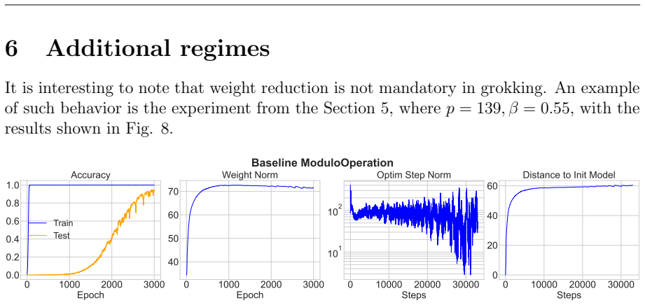
- [§6, Fig. 8] The observation that weight norm reduction is not mandatory in grokking is interesting but appears disconnected from the PPM discussion. A sentence linking it to the ravine/zero-risk-manifold picture would help.
Circularity Check
No definitional circularity in the reported speedup; main caveats are cost accounting of the pretraining phase and heavy reliance on the authors' own prior theoretical framing.
full rationale
The central quantitative claim is an external empirical comparison: PPM versus standard AdamW on ModuloOperation and MNIST, with both curves produced in this paper and accuracy thresholds defined independently of the method (Section 2: 99% test accuracy for ModuloOperation, 85% for MNIST). The reported 20x-100x acceleration is read off the ratio of epochs/gradient calls to the grokking threshold (Figs. 2, 4, 5), not computed from the interaction potential P(d)=A e^{-d/sigma} (Eq. 1). Eq. (1) is an update rule, not an estimator of grokking time, so no quantity being predicted is identical by construction to an input of the method. No fitted parameter is renamed as a prediction: the hyperparameters A, alpha_p, sigma, and N_d are chosen for the experiments, but the paper explicitly notes that a wide range of acceptable parameters speeds up training (comparing Figs. 4 and 6). The conceptual scaffolding (grokking as motion along a ravine, predator-prey direction as ravine direction, irreversibility via entropy) is inherited from the authors' own works [7,8,14]; the paper states that the PPM was 'introduced in [14,8]' and that the ravine picture was 'proposed' in [7,8]. This is a genuine self-citation chain, but it is not load-bearing for the measured numerical speedup, which is against an external AdamW baseline produced in the same paper. The paper's own admission that 'in practice it turned out to be more efficient to first training the model to achieve zero-risk manifold using the standard single-agent method' (Section 3) means the abstract's 'up to a hundred times faster learning' should be interpreted as acceleration of the grokking phase rather than end-to-end training from random initialization; this is a cost-accounting caveat, not circularity. Section 5's 'exponential law' is obtained by linear regression of log-epochs versus sample fraction, so calling it 'proven' is an overstatement, but it is a fit to data rather than a circular prediction derived from the method itself.
Assumptions & free parameters
free parameters (8)
- Interaction strength A =
150/15 (PP-stand), 1000/100 (PP-conn), 1500/150 (A > alpha_p)
- Predator rate alpha_p =
2A/3 in PP-stand (100 for ModuloOperation, 10 for MNIST); equal to A in PP-conn runs
- Interaction radius sigma =
10 (ModuloOperation), 1 or 10 (MNIST)
- Additional prey steps N_d =
5 for all reported runs
- GradPred flag =
False for the speedup runs; True for one illustrative run
- use_m (EMA of first moment) =
False for ModuloOperation PP-conn; True for MNIST PP-conn
- Initialization scale =
Embedding std=1.0 in Sections 2-4, std=0.02 in Section 5; MNIST weight multiplier unspecified
- Fitted scaling-law coefficients B, eta =
Not reported numerically
assumptions (5)
- domain assumption Ravine landscape model of grokking (zero-risk manifold, flat-bottomed ravines) from refs [7,8]
- ad hoc to paper Euclidean predator-prey displacement vector l_t indicates the ravine direction
- domain assumption Standard pre-training to the zero-risk manifold can be separated from the PPM phase and excluded from cost comparison
- ad hoc to paper Exponential and linear functional forms for grokking time
- ad hoc to paper Synchronized optimizer momenta between prey and predator preserve useful training dynamics
invented entities (1)
-
Predator and prey agents
Cite this review
Pith. "Pith review of Predator-Prey Model: Driven Hunt for Accelerated Grokking." pith.science (2026). https://pith.science/paper/2UYTV2JH
@misc{pith2026250910562,
  author       = {Pith},
  title        = {Pith review of: Predator-Prey Model: Driven Hunt for Accelerated Grokking},
  year         = {2026},
  howpublished = {\url{https://pith.science/paper/2UYTV2JH}},
  note         = {Machine review of arXiv:2509.10562}
}
read the original abstract
A machine learning method is proposed using two agents that simulate the biological behavior of a predator and a prey. In this method, the predator and the prey interact with each other - the predator chases the prey while the prey runs away from the predator - to perform an optimization on the landscape. This method allows, for the case of a ravine landscape (i.e., a landscape with narrow ravines and with gentle slopes along the ravines) to avoid getting optimization stuck in the ravine. For this, in the optimization over a ravine landscape the predator drives the prey along the ravine. Thus we also call this approach, for the case of ravine landscapes, the driven hunt method. For some examples of grokking (i.e., delayed generalization) problems we show that this method allows for achieving up to a hundred times faster learning compared to the standard learning procedure.
Figures


Figures from the paper (6 more)



Reference graph
Works this paper leans on
- [1]
-
[2]
Z. Liu, O. Kitouni, N. Nolte, E. J. Michaud, M. Tegmark, M. Williams, Towards Understanding Grokking: An Effective Theory of Representation Learning, NeurIPS 2022, arXiv:2205.10343
arXiv 2022
- [3]
-
[4]
Z. Liu, E. J. Michaud, M. Tegmark, Omnigrok: grokking beyond algorithmic data, Conference paper at ICLR 2023, arXiv:2210.01117
arXiv 2023
-
[5]
Z. Liu, A Good ML theory is Like Physics: A Physicist’s Analysis of Grokking, (2023), https://zimingliublog.wordpress.com/2023/06/16/a-good-ml-theory-is-like- physics-a-physicists-analysis-of-grokking/
work page 2023
- [6]
- [7]
-
[8]
S. V. Kozyrev, I. A. Lopatin, A. N. Pechen, Generalization in learning: Eyring for- mula and predator-prey model, Lobachevskii Journal of Mathematics, 46 (6), 2591– 2600 (2025). 14
work page 2025
Show all 23 references
-
[9]
I. M. Gelfand, M. L. Tsetlin, The principle of nonlocal search in automatic optimiza- tion systems, Dokl. Akad. Nauk SSSR, 137 (2), 295–298 (1961). [in Russian]
1961
-
[10]
I. M. Gelfand, M. L. Tsetlin, Some methods of control for complex systems, Russian Mathematical Surveys, 17 (1), 95–117 (1962)
1962
-
[11]
Nesterov, A method of solving a convex programming problem with convergence rateO(1/k 2), Soviet Mathematics Doklady, 27, 372–376 (1983)
Y. Nesterov, A method of solving a convex programming problem with convergence rateO(1/k 2), Soviet Mathematics Doklady, 27, 372–376 (1983)
1983
-
[12]
Fadili, From the Ravine method to the Nesterov method and vice versa: a dynamical system perspective, SIAM Journal on Optimization, 2022, 32 (3)
Hedy Attouch, Jalal M. Fadili, From the Ravine method to the Nesterov method and vice versa: a dynamical system perspective, SIAM Journal on Optimization, 2022, 32 (3)
2022
-
[13]
C. Liu, L. Zhu, M. Belkin, Loss landscapes and optimization in over-parameterized non-linear systems and neural networks, Applied and Computational Harmonic Anal- ysis, 59, 85–116 (2022). arXiv:2003.00307
2022 arXiv
-
[14]
S. V. Kozyrev, I. A. Lopatin, A. N. Pechen, Control of Overfitting with Physics, Entropy, 26, 1090 (2024). arXiv: 2412.10716
2024 arXiv
-
[15]
S. V. Albrecht, F. Christianos, and L. Sch¨ afer, Multi-Agent Reinforcement Learning, Foundations and Modern Approaches, The MIT Press, Cambridge, Massachusetts, London, England, 2024
2024
-
[16]
E. V. Koonin, The Logic of Chance: The Nature and Origin of Biological Evolution, FT Press, 2012
2012
-
[17]
Fisher, The Genetical Theory of Natural Selection, The Clarendon Press, UK, 1930
R. Fisher, The Genetical Theory of Natural Selection, The Clarendon Press, UK, 1930
1930
-
[18]
Kimura, The neutral theory of molecular evolution
M. Kimura, The neutral theory of molecular evolution. Cambridge University Press, (1983)
1983
-
[19]
Vaswani, N
A. Vaswani, N. Shazeer, N. Parmar, J. Uszkoreit, L. Jones, A. N. Gomez, L. Kaiser, I. Polosukhin, Attention Is All You Need, in: Advances in Neural Information Pro- cessing Systems 30 (NIPS 2017); arXiv:1706.03762v5
2017 arXiv
-
[20]
Loshchilov, F
I. Loshchilov, F. Hutter. 2019. Decoupled Weight Decay Regularization. arXiv: 1711.05101
2019 arXiv
-
[21]
A. Feng, A. Pechen, A. Jha, R. Wu, and H. Rabitz. 2012. Global Opti- mality of Fitness Landscapes in Evolution, Chem. Sci. 3 (3), 900–906 (2012). https://doi.org/10.1039/C1SC00648G
2012 doi
-
[22]
Pechen, Alexander N., and David J. Tannor. 2012. Quantum Control Landscape for a Λ–atom in the Vicinity of Second-Order Traps. Israel Journal of Chemistry 52 (5): 467–72. https://doi.org/10.1002/ijch.201100165
2012 doi
-
[23]
Volkov, Boris, Anastasia Myachkova, and Alexander Pechen. 2025. Phenomenon of a Stronger Trapping Behavior in Λ–Type Quantum Systems with Symmetry. Physical Review A 111 (2): 022617. https://doi.org/10.1103/PhysRevA.111.022617. 15
2025 doi
Reviewed August 4, 2026 · model on record in the stance chip above.
Discussion (0). Continue with ORCID to comment.