REVIEW 3 major objections 5 minor 12 references
An Empirical Study of Conjugate Gradient Preconditioners for Solving Symmetric Positive Definite Systems of Linear Equations
T0 review · 3 major / 5 minor · reviewed 2026-08-07 · deepseek-v4-flash
Pith's one-line read This benchmark of 108 preconditioner configurations on 79 symmetric positive definite matrices finds that incomplete Cholesky with AMD ordering yields the most consistent work reductions, with algebraic multigrid reliable but rarely…
desk verdict A careful, honestly reported benchmark with a genuinely new AMD-over-RCM result, but the abstract's blanket claim about SPD systems outruns the filtered test set. read the letter →
The pith
A machine-rendered reading of the paper's core claim, the machinery that carries it, and where it could break.
The reading
What carries the argument
The load-bearing measurement is the performance profile: for each preconditioner configuration, the fraction of test matrices where the total work, $\text{work} = (5n + \text{nonzeros} + \text{preconditioner})\cdot\text{iterations} + \text{preconditioner}$, is reduced by at least a factor $\tau$ relative to the diagonally scaled control, summarized by the area under the curve (AUC) in log2 space. Within that metric, the decisive object is the simplicial incomplete Cholesky factorization, which approximates $A \approx LL^T$ by keeping only entries above a drop tolerance; its best configuration combines threshold $10^{-8}$ with approximate minimum degree reordering. This object carries the argument because it alone combines large AUC with speedups of 2x or more on most of the test set, and because its generation-failure rate motivates the paper's call for fallback mechanisms.
What would settle it
Take the SPD matrices of dimension at least 10,000 from the same public sparse-matrix collection the paper used, keep only the ones that fail the $10n$ unpreconditioned-CG filter, and run the same 108 configurations with the same flop-based work metric. If IC/MIC's generation-success rate drops below the roughly 80% seen here, or if smoothed aggregation AMG achieves a higher AUC on that cohort, the paper's broad preference for incomplete Cholesky would not carry over to hard SPD systems.
Extended reading notes
Core claim
The paper's claim is that, over the class of SPD systems it can study, incomplete Cholesky is the most effective preconditioner class even when no per-matrix tuning is allowed. Under a single-best configuration, IC with drop tolerance $10^{-8}$ and AMD ordering achieves an AUC of 0.64, cuts total work by at least a factor of 2 on 78% of the 79 matrices, and reaches at least 8x on 62%; modified IC is close behind with AUC 0.61. Smoothed aggregation AMG, the best multigrid option, has AUC 0.36 and reaches 2x on only 38% of matrices, though it generates successfully on essentially all problems while IC and MIC fail to factor about 16-19% of the time. Classical SGS and SSOR preconditioners do not pay off, and unpreconditioned CG already beats an estimated direct solve by 2x on roughly 47% of matrices. The authors further claim that including construction cost shrinks but does not eliminate IC's edge, and that AMD ordering outperforms both RCM and natural orderings for incomplete factorizations, contradicting the usual preference for RCM.
Load-bearing premise
The whole comparison is run on a filtered set of SPD matrices where plain conjugate gradient converges within $10n$ iterations, so the conclusions about 'SPD systems' depend on that slice being representative; if the harder excluded matrices were added, incomplete factorizations would likely fail more often and the ranking could shift.
Editorial extensions
If this is right
- A user facing an SPD system where plain CG converges should try thresholded incomplete Cholesky with AMD ordering before anything else: the single-best IC configuration, drop tolerance $10^{-8}$ with AMD, gives at least a 2x work reduction on 78% of the benchmark matrices.
- Symmetric Gauss-Seidel and SSOR are a poor investment as black-box preconditioners; even their tuned variants produce large speedups on under 10% of problems.
- Algebraic multigrid is the most dependable fallback because it generates on 100% of test matrices and reaches parity with the baseline on 89-96%, even though its top speedups are smaller than IC's.
- Including preconditioner construction cost changes the practical message: with a single fixed configuration, only about 28% of problems retain a 4x total-work improvement, so per-matrix tuning or a build-cost-aware choice matters.
- Even the unpreconditioned baseline is competitive with direct solves on a large share of the test set, so direct solvers should not be assumed superior without measurement.
Reading between the lines
- Editorial inference: the $10n$ convergence filter likely biases the test set toward matrices where IC works, so the paper's headline claim should be read as 'IC is best among SPD systems that are already tractable for CG,' not as a universal SPD statement.
- Editorial inference: the work metric counts floating-point operations but not memory traffic or parallelism; a wall-clock study on multicore machines could narrow or reverse IC's margin over direct solvers, since sparse factorization is more parallelizable than the serial PCG recurrence.
- Editorial inference: the AMD-over-RCM result suggests a testable extension: compare IC with nested-dissection orderings at larger scales, where the authors' own data shows IC generation failing on 12 of the 16 largest matrices.
- Editorial inference: the success-parity numbers imply a natural hybrid strategy\u2014start with IC/AMD, fall back to AMG when generation or convergence fails\u2014that would likely combine IC's speed with AMG's near-universal reliability on this test set.
Signed reviews
Editorial analysis
A structured set of objections, weighed in public.
Referee Report
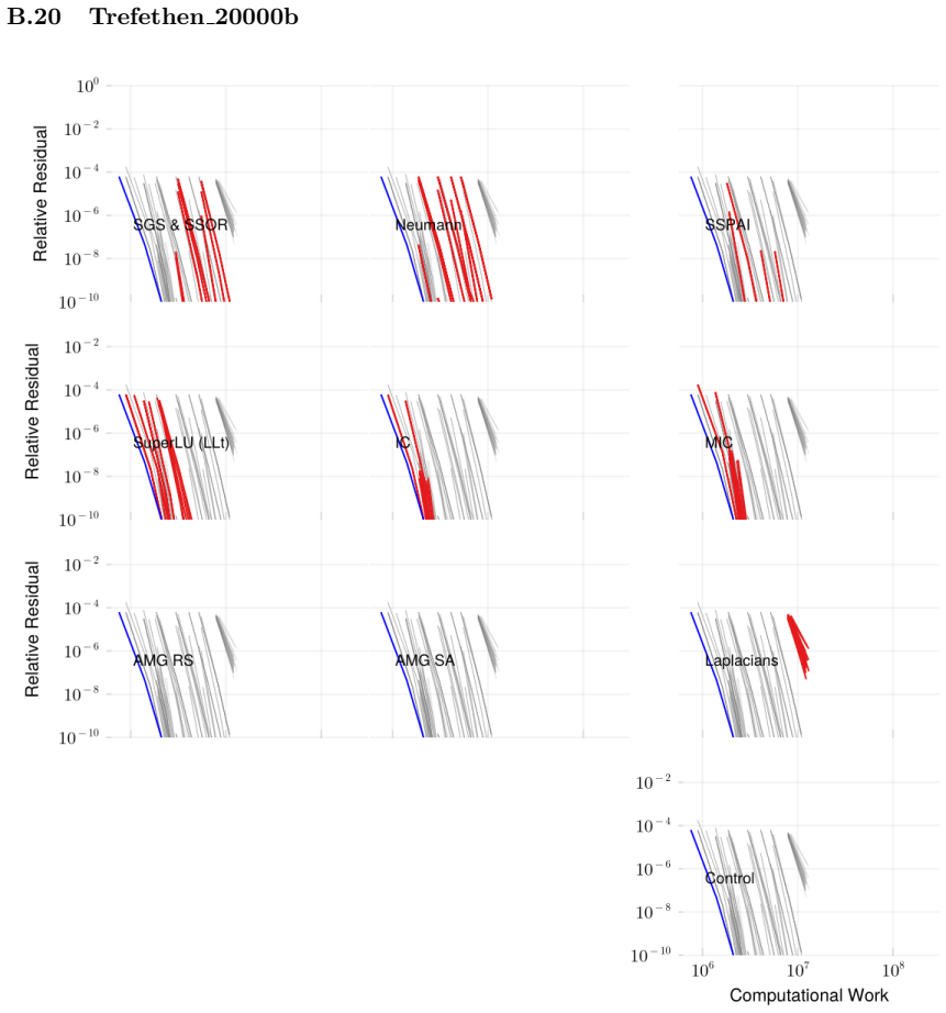
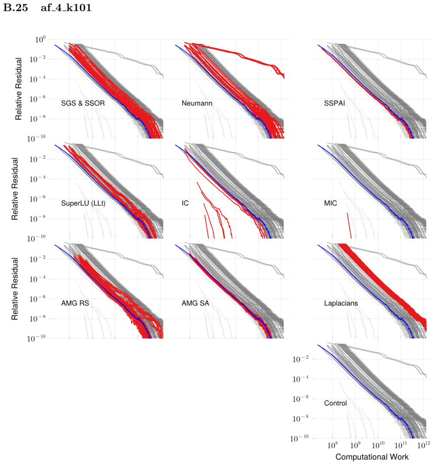
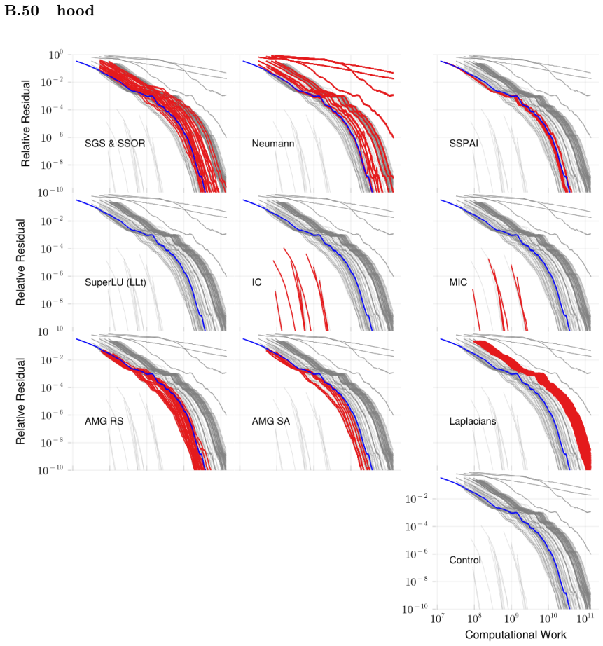
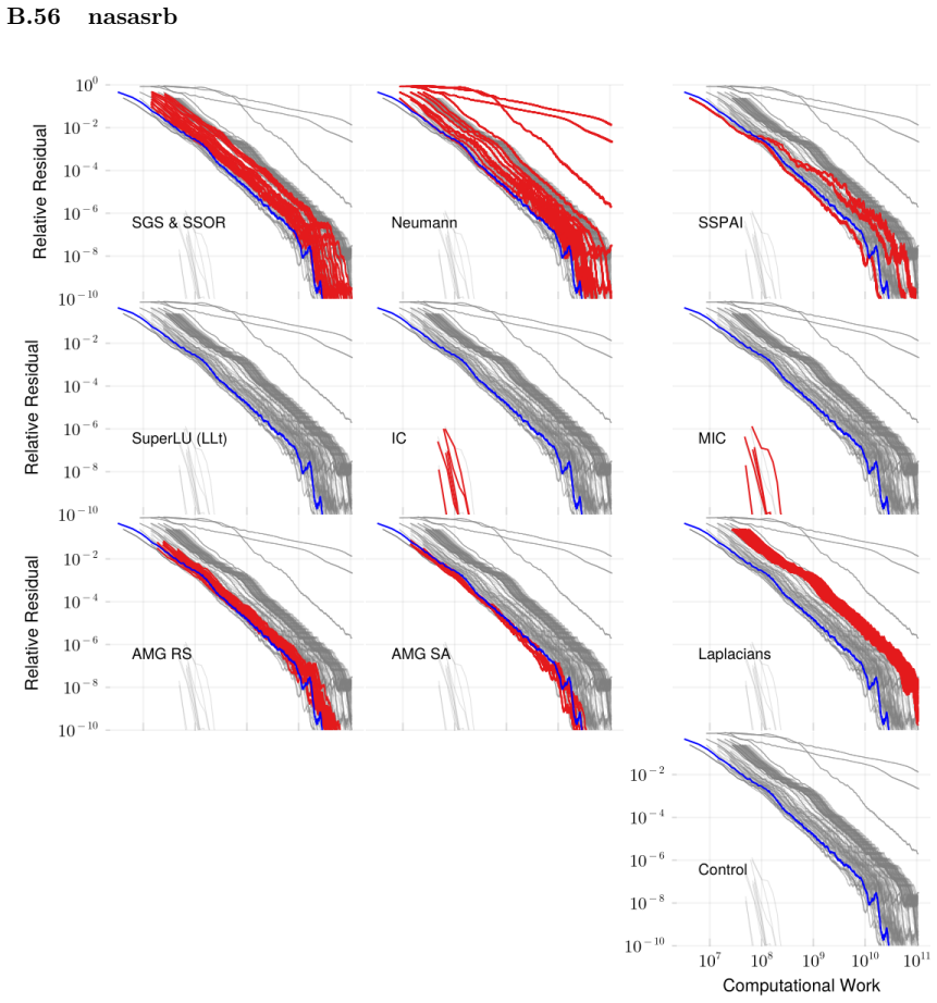
Summary. This paper presents an empirical benchmark of preconditioners for solving large sparse SPD systems with PCG. Using 79 SuiteSparse matrices of dimension at least 10,000, the authors evaluate 10 preconditioner classes in 108 configurations, reporting float-arithmetic work to reduce the relative residual to 1e-10 relative to a Jacobi-scaled unpreconditioned baseline and to an estimated sparse direct solve. The main reported findings are that incomplete Cholesky and modified incomplete Cholesky give the largest work reductions when they can be generated; AMG methods are reliable and occasionally strong; classical SGS/SSOR and SSPAI give little benefit; and including factorization construction costs substantially narrows the advantage over direct methods. The paper also studies the effect of AMD/RCM/natural orderings and of fill-in on incomplete factorizations, and it contains extensive per-matrix convergence plots in an appendix.
Significance. If the headline claims are taken as claims about the studied cohort, the paper is a useful and unusually transparent contribution: it covers a broad set of preconditioner families and configurations, documents the exact work metric, distinguishes single-best from per-matrix tuned choices, separates solve work from construction work, and provides reproducible code and data. The finding that AMD ordering consistently outperforms RCM for incomplete factorizations, contrary to some classical guidance, is interesting and worth reporting. However, the abstract and key findings generalize to 'symmetric positive definite systems' as a whole, while the experimental design explicitly filters to matrices where unpreconditioned CG already converges in at most 10n iterations and where the preconditioners can be generated. The in-sample selection of the 'single-best' configuration also makes the headline numbers optimistic. These issues are fixable with a revision that narrows the claims and adds robustness analysis.
major comments (3)
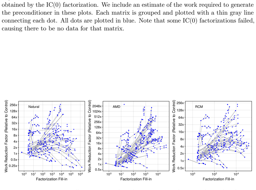
- [Abstract and §3] The abstract's headline claim, 'symmetric positive definite systems are mostly likely to benefit from incomplete symmetric factorizations,' is not supported for SPD systems in general. Section 5.1 restricts the test set to matrices for which unpreconditioned CG converges within 10n iterations, and footnote 1 says the remaining SPD matrices are still being studied. Section 3 then explicitly warns that concluding IC/MIC are the preferred preconditioners 'is premature' because they fail to generate on roughly 15–20% of problems and on 12 of the 16 largest matrices; Table 7 shows the best IC configuration has an 84% success rate. The evidence supports a claim about the filtered cohort, not about all SPD systems. The abstract and Section 3 should be reworded to state this conditionality, and the paper should at least discuss how the ranking might change if the excluded hard systems were included.
- [§2.2, §A.1, Table 7] The 'single-best configuration' is selected and evaluated on the same 79 matrices. Section 2.2 says the single-best configuration is chosen by computing the AUC over all matrices, and Section A.1 defines that AUC over the test set; the same data are then used to report the configuration's parity and 2x/4x/8x rates in Table 7 and Figure 4a. This is in-sample model selection and makes the headline numbers optimistic as estimates of how a fixed configuration would perform on new SPD systems. The authors should use a split or cross-validation for configuration selection, or otherwise quantify the selection bias, before presenting the single-best configuration as a practical recommendation.
- [Table 7 and §2.2] The central ranking of preconditioners rests on the AUC and on the geometric mean, where Table 7 defines failure to generate or converge as 4x control work. No sensitivity analysis is reported for this ad-hoc penalty, and the AUC can be dominated by a few very large speedups, so it is unclear whether the ordering 'IC best, AMG second' is robust. The paper should report additional distributional summaries (e.g., median work reduction, quantiles, and success rates alone) and show how the ranking changes if the 4x penalty is varied or if failed generations are treated as missing rather than as 4x control work.
minor comments (5)
- [Throughout] There are several typos and small wording errors: 'preconditoners' and 'mostly likely' in the abstract, 'availalbe' in Section 3.4, 'matric' in Section 5.3, 'T refethen' in Appendix B headings, and 'MC' instead of 'MIC' in Section 7.1.
- [§2.2] The sentence 'The best configurations for each method are summarized in Table 2' should refer to Table 7, since Table 2 lists preconditioner classes rather than configurations.
- [Table 7 caption] The caption defines 'Succ.' as the fraction of problems in which the preconditioner was successfully generated, but the geometric-mean definition also treats convergence failure as 4x control work; the caption should clarify whether 'Succ.' includes convergence failures after successful generation or only generation failures.
- [§2.3 and §2.6] The paper explicitly limits generation-cost comparisons to methods for which the cost can be estimated, and it correctly notes that AMG construction costs are not included. It would help to add a sentence in Section 3 making clear that the 'including generation cost' conclusions do not apply to AMG or to SSPAI.
- [§7.4] The table footnote for the AMG smoothed-aggregation entry states that one iteration of each cycle was best on 2.5% of the test set, but the wording is slightly confusing about whether the percentage refers to being tied for best; consider rewording for clarity.
Circularity Check
No significant circularity; the benchmark is an empirical measurement with disclosed in-sample selection and one minor non-load-bearing self-citation.
full rationale
This paper is an empirical benchmark, not a derivation chain, so most circularity patterns do not apply. The central claim that IC/MIC preconditioners give the largest work reduction is a measured ranking over a disclosed test set of 79 SPD matrices, computed from actual PCG convergence runs; it is not defined in terms of a fitted constant, nor does any equation make the conclusion true by construction. The single-best and tuned-best configurations are selected from the same test data (Section 2.2, Figures 4a/4b), but the paper explicitly labels them as in-sample selections rather than predictions, and it reports both to show sensitivity. The test-set filter requiring unpreconditioned CG convergence within 10n iterations (Section 5.1) and the footnote that the remaining SPD matrices are still being studied are scope limitations that affect generalizability, but they do not make the reported ranking circular: the inclusion criterion is about the unpreconditioned baseline, not about the success or ranking of the preconditioners being compared. The only self-citation is Gleich's GenericArpack.jl (reference in Section 4.2), used to compute the operator 2-norm for normwise backward error checking; that is a tool for convergence measurement, not a load-bearing premise for the IC-versus-AMG conclusion. No step reduces a prediction to its input by construction, no fitted parameter is renamed as a prediction, and no uniqueness theorem or ansatz is imported from the authors' prior work to force the choice of preconditioner. Accordingly, the appropriate finding is no significant circularity, with the score reflecting only the minor, non-load-bearing self-citation.
Assumptions & free parameters
free parameters (5)
- IC drop tolerance (best) =
1e-8 (with AMD ordering)
- AMG Smoothed Aggregation cycle (best) =
V-cycle, 1 iteration
- SSOR relaxation (best) =
omega = 1.2, 1 iteration
- SSPAI fill multiplier (best) =
2x average column count
- Failure penalty in geometric mean =
4x control
assumptions (6)
- domain assumption The 79 selected SuiteSparse matrices are representative of real-world SPD systems despite the filter that unpreconditioned CG converges within 10n iterations.
- domain assumption Floating-point operation count is an adequate proxy for computational cost.
- domain assumption The fill-based generation cost estimate approximates actual preconditioner construction work.
- domain assumption The seeded right-hand side generation produces convergence behavior representative of generic RHS vectors.
- ad hoc to paper Failure to generate or converge is assigned 4x control work in the geometric mean metric.
- standard math Standard PCG, SPD matrix theory, and Dolan-More performance profile methodology are accepted background.
Cite this review
Pith. "Pith review of An Empirical Study of Conjugate Gradient Preconditioners for Solving Symmetric Positive Definite Systems of Linear Equations." pith.science (2026). https://pith.science/paper/2XN2KFBT
@misc{pith2026250520696,
  author       = {Pith},
  title        = {Pith review of: An Empirical Study of Conjugate Gradient Preconditioners for Solving Symmetric Positive Definite Systems of Linear Equations},
  year         = {2026},
  howpublished = {\url{https://pith.science/paper/2XN2KFBT}},
  note         = {Machine review of arXiv:2505.20696}
}
read the original abstract
Despite hundreds of papers on preconditioned linear systems of equations, there remains a significant lack of comprehensive performance benchmarks comparing various preconditioners for solving symmetric positive definite (SPD) systems. In this paper, we present a comparative study of 79 matrices using a broad range of preconditioners. Specifically, we evaluate 10 widely used preconditoners across 108 configurations to assess their relative performance against using no preconditioner. Our focus is on preconditioners that are commonly used in practice, are available in major software packages, and can be utilized as black-box tools without requiring significant \textit{a priori} knowledge. In addition, we compare these against a selection of classical methods. We primarily compare them without regards to effort needed to compute the preconditioner. Our results show that symmetric positive definite systems are mostly likely to benefit from incomplete symmetric factorizations, such as incomplete Cholesky (IC). Multigrid methods occasionally do exceptionally well. Simple classical techniques, symmetric Gauss Seidel and symmetric SOR, are not productive. We find that including preconditioner construction costs significantly diminishes the advantages of iterative methods compared to direct solvers; although, tuned IC methods often still outperform direct methods. Additionally, ordering strategies such as approximate minimum degree significantly enhance IC effectiveness. We plan to expand the benchmark with larger matrices, additional solvers, and detailed metrics to provide actionable information on SPD preconditioning.
Figures


Figures from the paper (93 more)
















Reference graph
Works this paper leans on
-
[8]
Cited on page 21. M.Ferronato, C.Janna, and G.Pini.Shifted fsai preconditioners for the efficient parallel solu- tion of non-linear groundwater flow models. In- ternational Journal for Numerical Methods in Engineering, 89 (13), p. 1707–1719, 2011. doi: 10.1002/nme.3309. Cited on page 21. Y.Gao, R.Kyng, and D. A.Spielman.Robust and practical solution of la...
-
[11]
doi:10.1016/j.parco.2008.12.006. Cited on page 21. P.Wissgott.Wissgott group. https://sparse.tamu. edu/Wissgott, 2007. Vienna University of Technol- ogy. Includes parabolic fem. Retrieved from SuiteS- parse. Cited on page 21. D. M.Young.The rate of convergence of an improved iterative method for solving the finite difference ana- logue of the dirichlet pr...
-
[1954]
Cited on pages 2, 24, and 25. 39 Appendix §ASupplemental details41 A.1 AUC calculation for performance profiles 41 A.2 Generation cost for incomplete factoriza- tions and sparse direct methods41 §B All Problems Convergence Results41 B.1 2cubes sphere42 B.2 BenElechi143 B.3 Bump 291144 B.4 Dubcova145 B.5 Dubcova246 B.6 Dubcova347 B.7 Emilia 92348 B.8 Fault...
-
[1977]
doi:10.1090/s0025-5718-1977-0438681-4 . Cited on pages 2 and 26. U.Okuyucu.Amd group. https://sparse.tamu. edu/AMD, 2006. AMD, Inc. Includes G2 circuit and G3 circuit. Retrieved from SuiteSparse. Cited on page 21. D.Orban.Limited-memory ldlt factorization of symmetric quasi-definite matrices with applica- tion to constrained optimization. Numerical Al- go...
-
[1996]
A Simple, Combinatorial Algorithm for Solving SDD Systems in Nearly-Linear Time
Cited on page 27. R.Grimes.Boeing group. https://sparse.tamu. edu/Boeing, 1995. Boeing. Includes crystm02 and crystm03. Retrieved from SuiteSparse. Cited on page 21. M. J.Groteand T.Huckle.Parallel preconditioning with sparse approximate inverses. SIAM Journal on Scientific Computing, 18 (3), p. 838–853, 1997. doi:10.1137/s1064827594276552. Cited on page ...
work page Pith review arXiv doi:10.48550/arxiv.1301.6628 1995
-
[2001]
doi:10.1007/s211-001-8015-y . Cited on page 27. J.Weiher.Inpro group. https://sparse.tamu.edu/ INPRO, 2005. Includes matrices from project PARA- SOL. Includes msdoor. Retrieved from SuiteSparse. Cited on page 21. S.Williams, L.Oliker, R.Vuduc, J.Shalf, K.Yelick, and J.Demmel.Optimization of sparse matrix–vector multiplication on emerging multicore platfor...
-
[2003]
Cited on page 22. T.George, A.Gupta, and V.Sarin.An em- pirical analysis of the performance of precondi- tioners for spd systems. ACM Transactions on 36 Mathematical Software, 38 (4), p. 1–30, 2012. doi:10.1145/2331130.2331132. Cited on page 2. A.Ghai, C.Lu, and X.Jiao.A comparison of preconditioned krylov subspace methods for large- scale nonsymmetric li...
-
[2005]
Cited on page 26. X. S.Liand M.Shao.A supernodal approach to incomplete LU factorization with partial pivoting. ACM Trans. Mathematical Software, 37 (4), 2010. Cited on page 26. M.Lourakis.Lourakis group. https://sparse.tamu. edu/Lourakis, 2006. Foundation for Research and Technology Hellas — Institute of Computer Sci- ence. Includes bundle1. Retrieved fr...
work page 2010
Show all 12 references
-
[2008]
Includes cbuckle and smt
Helsinki University of Technology. Includes cbuckle and smt. Retrieved from SuiteSparse. Cited on page 21. P.Krysl.Symrcm: Reverse cuthill- mckee node-renumbering algorithm. https://github.com/PetrKryslUCSD/SymRCM.jl,
-
[2009]
In- cludes shallow water1 and shallow water2
Max-Planck Institute of Meteorology. In- cludes shallow water1 and shallow water2. Re- trieved from SuiteSparse. Cited on page 21. N.Li, Y.Saad, and E.Chow.Crout versions of ilu for general sparse matrices. SIAM Journal on Scientific Computing, 25 (2), p. 716–728, 2003. doi:10...
2003 doi
-
[2011]
15This preconditioner was invariant to ordering
Cited on pages 2, 26, and 27. 15This preconditioner was invariant to ordering. One iteration of each cycle were each either the best overall preconditioner or tied with the best on 2 .5% of the test set. Performing a single iteration of the preconditioner tended to be the best...
-
[2020]
Cited on page 22
Commit ae805a8c01b0aeaaaf6040f0f91ca862f032311a. Cited on page 22. 37 R. B.Lehoucq, D. C.Sorensen, and C.Yang. ARPACK Users’ Guide: Solution of Large-Scale Eigenvalue Problems with Implicitly Restarted Arnoldi Methods, Society for Industrial and Applied Mathematics, 1998. doi:...
1998 doi
Reviewed August 7, 2026 · model on record in the stance chip above.
Discussion (0). Continue with ORCID to comment.