REVIEW 4 major objections 4 minor 48 references
Incorporating Correlated Nugget Effects in Multivariate Spatial Models: An Application to Argo Ocean Data
T0 review · 4 major / 4 minor · reviewed 2026-08-07 · deepseek-v4-flash
Pith's one-line read Adding a correlated nugget to bivariate spatial models lowers the estimated median temperature–salinity correlation from 0.95 to 0.87 in global ocean profile data.
desk verdict A solid methodological extension whose headline oceanographic claim—systematic overestimation of latent T–S correlation—rests on an identifiability assumption that is plausible but not demonstrated; worth refereeing with a request for revision. read the letter →
The pith
A machine-rendered reading of the paper's core claim, the machinery that carries it, and where it could break.
The reading
What carries the argument
The central object is a bivariate Matérn-SPDE field whose smooth cross-dependence is controlled by a dependence matrix $\mathbf{D}(\theta,\rho)$, paired with an observation model whose noise covariance at co-located points is $\boldsymbol{\Sigma}_\varepsilon=\begin{pmatrix}\sigma_{\varepsilon,1}^2 & \sigma_{\varepsilon,1}\sigma_{\varepsilon,2}\rho_\varepsilon\\ \sigma_{\varepsilon,1}\sigma_{\varepsilon,2}\rho_\varepsilon & \sigma_{\varepsilon,2}^2\end{pmatrix}$. The argument is carried by the split between $\rho$ and $\rho_\varepsilon$: setting $\rho_\varepsilon=0$ forces $\rho$ to absorb all cross-variable dependence, whereas the general model lets small-scale shared noise account for part of it. Proposition 2.1 converts $\rho$ into a Pearson correlation for the $\alpha=2$, $d=2$ case, and that conversion is what the empirical comparisons use.
What would settle it
Fit the correlated- and independent-nugget models to paired temperature and salinity profiles restricted to the most accurately calibrated floats, so the measurement-noise variance is very small; if the latent correlation drop from about 0.95 to 0.87 persists, it is a real field property, but if the drop shrinks toward zero, the headline comparison is dominated by the very measurement noise the model adds.
Extended reading notes
Core claim
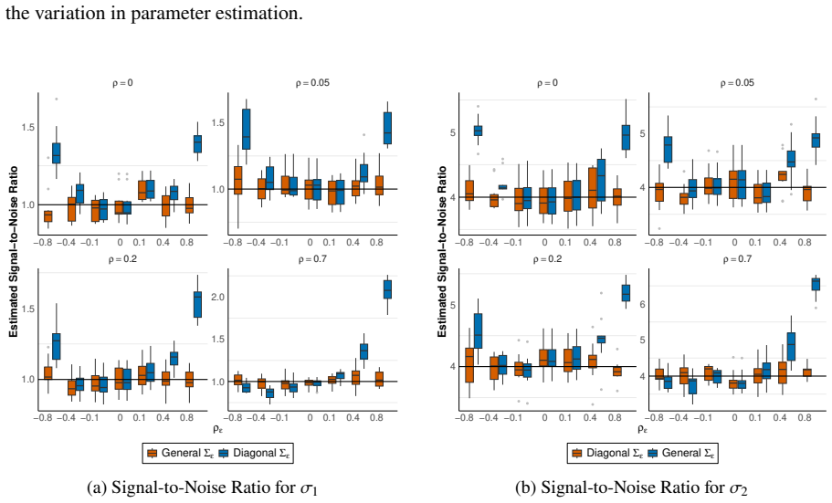
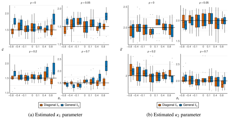
The central claim is that, when two variables are observed at the same location, the shared component of their small-scale noise should be estimated as a parameter rather than forced to zero. The authors define a bivariate process $\mathbf{X}(s)=\mathbf{m}(s)+\mathbf{u}(s)$ with latent cross-dependence governed by a parameter $\rho$ and add a nugget covariance whose off-diagonal element $\rho_\varepsilon$ carries correlated measurement error. Across simulation settings with known $\rho$, they show that fitting with $\rho_\varepsilon=0$ biases the estimated dependence—with $\rho_\varepsilon=-0.8$ turning a true $\rho=0$ into an estimate near $-0.5$—while fitting with the general nugget recovers it. Applied to temperature and salinity at 300 dbar, the fitted dependence parameter $\rho$ falls from 4.90 to 2.30 in the Gaussian model and from 3.96 to 2.19 in the NIG model, and the fitted $\rho_\varepsilon$ is uniformly large and positive. The authors interpret the drop as evidence that independent-noise analyses absorbed measurement coincidence into the latent field.
Load-bearing premise
The load-bearing premise is that the model can tell apart a shared, same-location noise component from a smooth genuine correlation between the two fields; if those two are not separately identifiable from the likelihood, the reported drop in latent correlation is mostly a bookkeeping change.
Editorial extensions
If this is right
- Gridded ocean products built with independent measurement errors would inherit overstated temperature–salinity coupling, so derived quantities such as potential density and steric-height estimates would carry that bias.
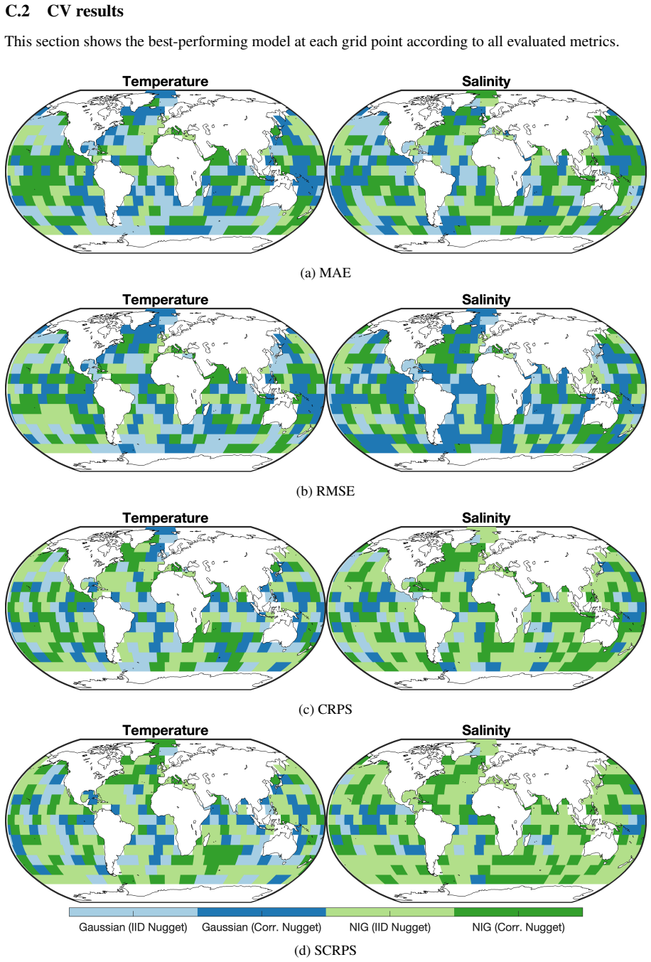
- At 300 dbar, the Gaussian correlated-nugget model attains the best leave-one-out predictive scores for temperature and salinity, showing the extra parameter earns its keep in prediction.
- Once nugget correlation is included, the non-Gaussian NIG model offers little improvement over the Gaussian model at 300 dbar, suggesting part of the apparent non-Gaussianity was a misfit symptom of the uncorrelated-noise assumption.
- Because fitted nugget correlations are typically above 0.7 in the ocean-profile application, the distorting effect of assuming independence is strongest in the exact regime where the data are most noise-coupled.
Reading between the lines
- Editorial inference: paired environmental sensors with shared platform or calibration noise—temperature–oxygen or salinity–nitrate float pairs—should show the same inflation when fitted with diagonal nuggets, so the practice of independent-nugget multivariate spatial modeling deserves scrutiny outside oceanography.
- A direct test not run in the paper: for floats surfacing within a few kilometers of each other, treat the difference of co-located readings as an empirical nugget and compare it with the fitted $\rho_\varepsilon$ at the same pressure level.
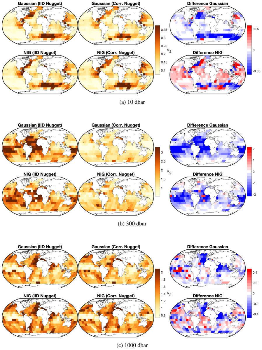
- Because the 1000 dbar maps show heterogeneous signs, extending the mechanism to nonstationary or three-dimensional SPDEs should re-examine whether the roughly 0.08 drop in latent correlation is uniform across depth and latitude.
Editorial analysis
A structured set of objections, weighed in public.
Referee Report
Summary. The paper proposes bivariate Gaussian and NIG Matérn-SPDE models with a correlated nugget component, estimated by maximum likelihood or stochastic gradient methods, and applies them with a moving-window design to Argo temperature and salinity at 10, 300, and 1000 dbar. The central empirical claim is that adding a nugget correlation parameter lowers the estimated latent temperature–salinity correlation (at 300 dbar, the median Pearson correlation drops from 0.95 to 0.87 in the Gaussian model and from 0.94 to 0.87 in the NIG model), which the authors interpret as evidence that traditional independent-nugget models overstate the underlying field correlation. The paper also includes a simulation study with 42 configurations and 10 replicates, LOOCV tables, QQ diagnostics, and an open-source implementation in the ngme2 R package.
Significance. The paper addresses a real and important problem in oceanographic mapping and multivariate geostatistics. The methodological package has clear strengths: an open-source implementation, reproducible code and data, an analytic mapping from the dependence parameter to the Pearson correlation (Proposition 2.1), a systematic simulation grid, and evaluation with proper scoring rules and LOOCV. If the interpretation of the fitted nugget correlation as measurement-error correlation were established, the paper would be a useful caution for Argo gridded products. However, as written, the headline claim is load-bearing on an identifiability and interpretation assumption that is not demonstrated, and the paper's own 1000 dbar results contradict the 'systematically overstates' phrasing. The central result is therefore defensible but requires additional support or substantial qualification.
major comments (4)
- [Section 4 and Section 5.3] The split between the correlated nugget and the latent cross-dependence is not shown to be identifiable. The total co-located covariance is Sigma_u(0) + Sigma_epsilon, so the nugget is separated from the latent field only by extrapolating the smooth alpha=2 Matérn covariance to zero lag. The simulation study in Section 4 always generates data with nonzero rho_epsilon and never includes the null case rho_epsilon = 0, so it cannot rule out the possibility that the general model spuriously estimates a nonzero nugget correlation and shrinks rho. I recommend adding a null-configuration simulation (rho_epsilon = 0) and a profile-likelihood or similar identifiability check before the Section 5.3 interpretation of the rho drop is used as evidence.
- [Section 2.1 and Section 5.3] The interpretation of the fitted rho_epsilon as 'measurement-error correlation' is an interpretive leap relative to the model definition. In Section 2.1, the nugget is explicitly defined as 'measurement noise and small-scale variability,' so a well-identified rho_epsilon can absorb spatially white physical covariability between temperature and salinity at sub-window scales. In that case, the observed reduction in the latent dependence parameter rho is a scale-decomposition artifact rather than a correction for sensor error. The paper needs either external evidence tying rho_epsilon to Argo sensor error characteristics or a model that separates the small-scale process from measurement noise before claiming that traditional models overestimate the underlying field correlation.
- [Section 5.3 and Figure 7] The claim that ignoring measurement-error correlation 'systematically overstates between-field dependence' is contradicted by the paper's own results at other depths. At 1000 dbar, most grid cells display a positive difference (correlated minus independent), and at 10 dbar the equatorial region reverses, with correlations up to 0.15 higher under the correlated model. The abstract and conclusions should be qualified to depth-specific or region-specific statements, or the global claim should be supported by a summary statistic that accounts for the heterogeneity shown in Figure 7.
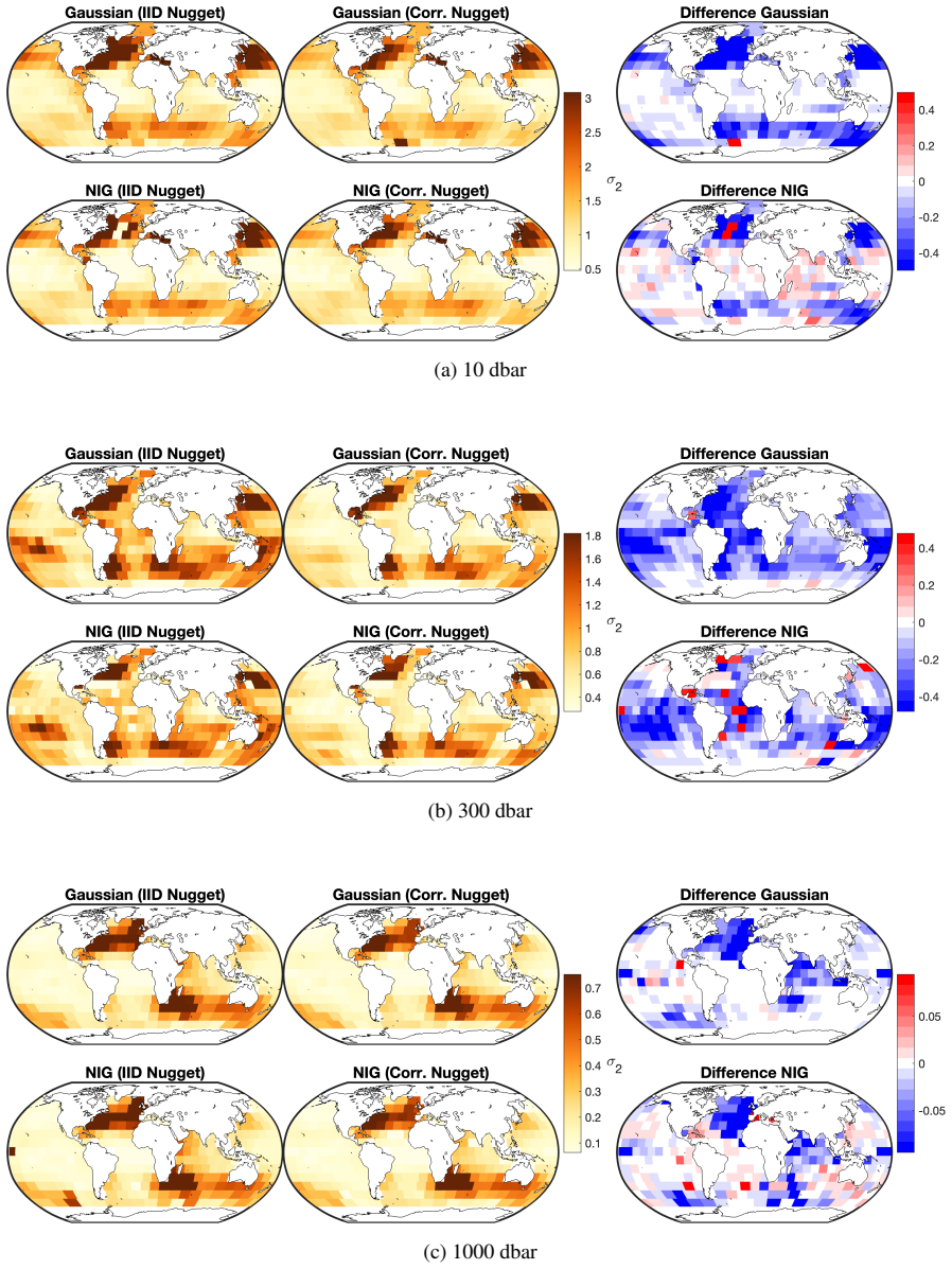
- [Section 5.3 and Figures 5-8] The reported median correlations and parameter maps are point estimates from many moving-window optimizations, with no standard errors, confidence intervals, or sensitivity analysis. Without uncertainty quantification, the apparent drop in latent correlation (0.95 to 0.87 at 300 dbar) cannot be distinguished from estimation noise, and the abstract's claim of 'significantly improves' is not statistically supported. At minimum, the paper should report uncertainty for the window-level parameter estimates or provide a bootstrap/ensemble analysis.
minor comments (4)
- [Section 3.2, Eq. (11)] The constant term in the log-likelihood is written as '-N1 log(2π)', but the likelihood is over all N observations; this should presumably be -(N/2)log(2π) or the notation for N1 should be clarified.
- [Section 3.1 and Appendix B.1] The correlated nugget precision in Eq. (17) is written for N1 = N2 = n with observations at the same locations, while the model statement in Eq. (10) allows different locations for the two fields. The paper should clarify how Q_epsilon is defined when the two variables are not co-located or only partially co-located within a window.
- [References] References [1] and [2] contain duplicated page ranges (e.g., 'pp. 283–312, pp. 283–312'); the bibliography should be cleaned.
- [Appendix C.4 and Figure 2] The boxplots display only selected values of the true latent correlation (rho = 0, 0.05, 0.2, 0.7); either all seven simulated configurations should be shown or the caption should state why the omitted ones are excluded.
Circularity Check
No significant circularity: the drop in latent correlation is an estimated outcome of fresh model fits, not an input or a reparameterization that forces the conclusion.
full rationale
The paper's central claim is that adding a correlated nugget lowers the estimated latent temperature–salinity correlation in Argo data. This claim is not equivalent to any input by construction. The latent correlation parameter rho and the nugget correlation parameter rho_epsilon are both free parameters estimated from Argo residuals by maximum likelihood or stochastic gradient; the model permits rho_epsilon = 0 but estimates large positive values, and the resulting drop in rho, and in the Proposition 2.1 Pearson correlation, is a fitted outcome rather than an imposed constraint. Proposition 2.1 is a mathematical derivation that converts fitted parameters into a Pearson correlation, not a redefinition of the result. The simulation study generates data from the same bivariate SPDE family and shows that a diagonal-nugget fit is biased when the true nugget is correlated; this is a standard self-consistency check with known truth, and the paper supplements it with leave-one-out cross-validation on real Argo data, which is genuinely out-of-sample. Self-citations to Bolin and Wallin (2018, 2023) and to the ngme2 package supply the SPDE machinery, Gibbs sampler, and scoring-rule estimators; those prior results are published, code-reproduced, and do not themselves contain the Argo finding, so the citations are not load-bearing in a circular way. The remaining concern, that the correlated nugget may not be separately identifiable from the latent cross-covariance or may absorb real small-scale physical variability rather than measurement error, is a modeling and identifiability risk rather than a circularity of the derivation chain.
Assumptions & free parameters
free parameters (10)
- alpha1=alpha2 smoothness =
2 (fixed)
- rho latent dependence parameter
- rho_epsilon nugget correlation
- sigma_epsilon_1, sigma_epsilon_2
- kappa_1, kappa_2
- sigma_1, sigma_2
- eta_1, eta_2
- mu_1, mu_2
- beta regression coefficients
- window margin and grid dimensions =
10x10 grid; 5-degree margin
assumptions (7)
- standard math Gaussian Matérn fields solve the SPDE in equation (3) with the stated normalization.
- standard math Finite-element Galerkin solution on a bounded domain with Neumann boundary conditions approximates the R^d SPDE solution.
- standard math NIG and generalized asymmetric Laplace noises are the convolution-closed subclasses needed for SPDE models.
- domain assumption Within each 20 by 20 degree moving window, the bivariate field is stationary and the latent parameters are constant.
- domain assumption January data from different years are treated as independent replicates after local polynomial mean removal.
- domain assumption The correlated nugget and the smooth latent cross-correlation are identifiable from the bivariate observations.
- standard math Stochastic approximation converges under the chosen weight sequence.
Cite this review
Pith. "Pith review of Incorporating Correlated Nugget Effects in Multivariate Spatial Models: An Application to Argo Ocean Data." pith.science (2026). https://pith.science/paper/3CTDK3G7
@misc{pith2026250603042,
  author       = {Pith},
  title        = {Pith review of: Incorporating Correlated Nugget Effects in Multivariate Spatial Models: An Application to Argo Ocean Data},
  year         = {2026},
  howpublished = {\url{https://pith.science/paper/3CTDK3G7}},
  note         = {Machine review of arXiv:2506.03042}
}
read the original abstract
Accurate analysis of global oceanographic data, such as temperature and salinity profiles from the Argo program, requires geostatistical models capable of capturing complex spatial dependencies. This study introduces Gaussian and non-Gaussian hierarchical multivariate Mat\'ern-SPDE models with correlated nugget effects to account for small-scale variability and measurement error correlations. Using simulations and Argo data, we demonstrate that incorporating correlated nugget effects significantly improves the accuracy of parameter estimation and spatial prediction in both Gaussian and non-Gaussian multivariate spatial processes. When applied to global ocean temperature and salinity data, our model yields lower correlation estimates between fields compared to models that assume independent noise. This suggests that traditional models may overestimate the underlying field correlation. By separating these effects, our approach captures fine-scale oceanic patterns more effectively. These findings show the importance of relaxing the assumption of independent measurement errors in multivariate hierarchical models.
Figures


Figures from the paper (29 more)








Reference graph
Works this paper leans on
-
[1]
Stability of Stochastic Approximation under Verifiable Condi- tions
Christophe Andrieu, Éric Moulines, and Pierre Priouret. “Stability of Stochastic Approximation under Verifiable Condi- tions”.SIAM Journal on Control and Optimization44 pp. 283–312, pp. 283–312.doi:10.1137/S0363012902417267
-
[3]
Argo data management Team.Argo user’s manual. Report. 2022.doi:10.13155/29825
-
[4]
Linear Mixed Effects Models for Non-Gaussian Continuous Repeated Measurement Data
Özgür Asar, David Bolin, Peter J. Diggle, and Jonas Wallin. “Linear Mixed Effects Models for Non-Gaussian Continuous Repeated Measurement Data”.Journal of the Royal Statistical Society Series C: Applied Statistics69 pp. 1015–1065, pp. 1015–1065.doi:10.1111/rssc.12405
-
[5]
PressuresensordriftsinArgoandtheirimpacts
PaulM.Barker,JeffR.Dunn,CatiaM.Domingues,andSusanE.Wijffels.“PressuresensordriftsinArgoandtheirimpacts”. Journal of Atmospheric and Oceanic Technology28 pp. 1036–1049, pp. 1036–1049.doi:10.1175/2011JTECHO831.1
-
[6]
Normal Inverse Gaussian Distributions and Stochastic Volatility Modelling
Ole E. Barndorff-Nielsen. “Normal Inverse Gaussian Distributions and Stochastic Volatility Modelling”.Scandinavian Journal of Statistics24 pp. 1–13, pp. 1–13
-
[7]
Introduction to optimal interpolation and variational analysis
Alexander Barth, Aida Alvera Azcárate, Pascal Joassin, Jean-Marie Beckers, and Charles Troupin. “Introduction to optimal interpolation and variational analysis”.SESAME Summer School, Varna, Bulgaria
-
[8]
Spatial Matérn fields driven by non-Gaussian noise
David Bolin. “Spatial Matérn fields driven by non-Gaussian noise”.Scandinavian Journal of Statistics41 pp. 557–579, pp. 557–579.doi:10.1111/sjos.12046
-
[9]
R package version 0.6.0, https://github.com/davidbolin/ngme2
David Bolin, Xiaotian Jin, Alexandre Simas, and Jonas Wallin.ngme2: Latent Mixed Effects Models with Flexible Distributions. R package version 0.6.0, https://github.com/davidbolin/ngme2. 2024
work page 2024
Show all 48 references
-
[10]
TheRationalSPDEApproachforGaussianRandomFieldsWithGeneralSmoothness
DavidBolinandKristinKirchner.“TheRationalSPDEApproachforGaussianRandomFieldsWithGeneralSmoothness”. Journal of Computational and Graphical Statistics29 pp. 274–285, pp. 274–285.doi:10.1080/10618600.2019. 1665537
2019
-
[11]
Covariance–Based Rational Approximations of Fractional SPDEs for Computationally Efficient Bayesian Inference
David Bolin, Alexandre B. Simas, and Zhen Xiong. “Covariance–Based Rational Approximations of Fractional SPDEs for Computationally Efficient Bayesian Inference”.Journal of Computational and Graphical Statistics33 pp. 64–74, pp. 64–74.doi:10.1080/10618600.2023.2231051
-
[12]
Multivariate type G Matérn stochastic partial differential equation random fields
David Bolin and Jonas Wallin. “Multivariate type G Matérn stochastic partial differential equation random fields”. Journal of the Royal Statistical Society. Series B: Statistical Methodology82.doi:10.1111/rssb.12351
-
[13]
Local scale invariance and robustness of proper scoring rules
David Bolin and Jonas Wallin. “Local scale invariance and robustness of proper scoring rules”.Statistical Science38 pp. 140–159, pp. 140–159.doi:10.1214/22-STS864
-
[14]
A technique for objective analysis and design of oceanographic experiments applied to MODE-73
Francis P. Bretherton, Russ E. Davis, and C.B. Fandry. “A technique for objective analysis and design of oceanographic experiments applied to MODE-73”.Deep Sea Research and Oceanographic Abstracts23 pp. 559–582, pp. 559–582.doi: 10.1016/0011-7471(76)90001-2
-
[15]
An assessment of oceanic variability for 1960–2010 from the GFDL ensemble coupled data assimilation
You-Soon Chang, Shaoqing Zhang, Anthony Rosati, Thomas L. Delworth, and William F. Stern. “An assessment of oceanic variability for 1960–2010 from the GFDL ensemble coupled data assimilation”.Climate Dynamics40 pp. 775–803, pp. 775–803
1960
-
[16]
Wikle.Statistics for Spatio-Temporal Data
Noel Cressie and Christopher K. Wikle.Statistics for Spatio-Temporal Data. New York, NY: John Wiley & Sons, 2011
2011
-
[17]
Maximum Likelihood from Incomplete Data Via the EM Algorithm
A. P. Dempster, N. M. Laird, and D. B. Rubin. “Maximum Likelihood from Incomplete Data Via the EM Algorithm”. Journal of the Royal Statistical Society: Series B (Methodological)39 pp. 1–22, pp. 1–22.doi:https://doi.org/10. 1111/j.2517-6161.1977.tb01600.x
-
[18]
Ocean Salinities Reveal Strong Global Water Cycle Intensification During 1950 to 2000
Paul J. Durack, Susan E. Wijffels, and Richard J. Matear. “Ocean Salinities Reveal Strong Global Water Cycle Intensification During 1950 to 2000”.Science336 pp. 455–458, pp. 455–458.doi:10.1126/science.1212222
1950 doi
-
[19]
Does non-stationary spatial data always require non-stationary random fields?
Geir-Arne Fuglstad, Daniel Simpson, Finn Lindgren, and Håvard Rue. “Does non-stationary spatial data always require non-stationary random fields?”Spatial Statistics14 pp. 505–531, pp. 505–531.doi:https://doi.org/10.1016/j. spasta.2015.10.001
-
[20]
Quality Control of Large Argo Datasets
F. Gaillard et al. “Quality Control of Large Argo Datasets”.Journal of Atmospheric and Oceanic Technology26 pp. 337–351, pp. 337–351.doi:10.1175/2008JTECHO552.1
-
[21]
In-situ based reanalysis of the global ocean temperature and salinity with ISAS: variability of the heat content and steric height
Fabienne Gaillard, Thierry Reynaud, Virginie Thierry, Nicolas Kolodziejczyk, and Karina von schuckmann. “In-situ based reanalysis of the global ocean temperature and salinity with ISAS: variability of the heat content and steric height”. Journal Of Climate29 pp. 1305–1323, pp....
-
[22]
Spatial statistics and Gaussian processes: A beautiful marriage
Alan E. Gelfand and Erin M. Schliep. “Spatial statistics and Gaussian processes: A beautiful marriage”.Spatial Statistics 18 pp. 86–104, pp. 86–104.doi:10.1016/j.spasta.2016.03.006
2016 doi
-
[23]
Estimating oxygen in the Southern Ocean using Argo temperature and salinity
D. Giglio, V. Lyubchich, and M. R. Mazloff. “Estimating oxygen in the Southern Ocean using Argo temperature and salinity”.Journal of Geophysical Research: Oceans123 pp. 4280–4297, pp. 4280–4297.doi:10.1029/2017jc013404
-
[24]
MatérnCross-CovarianceFunctionsforMultivariateRandom Fields
TilmannGneiting,WilliamKleiber,andMartinSchlather.“MatérnCross-CovarianceFunctionsforMultivariateRandom Fields”.Journal of the American Statistical Association105.doi:10.1198/jasa.2010.tm09420. 40
2010 doi
-
[25]
Strictly proper scoring rules, prediction, and estimation
Tilmann Gneiting and Adrian E. Raftery. “Strictly proper scoring rules, prediction, and estimation”.Journal of the American Statistical Association102 pp. 359–378, pp. 359–378.doi:10.1198/016214506000001437
-
[26]
Lognormal and Moving Window Methods of Estimating Acid Deposition
Timothy C. Haas. “Lognormal and Moving Window Methods of Estimating Acid Deposition”.Journal of the American Statistical Association85 pp. 950–963, pp. 950–963.doi:10.1080/01621459.1990.10474966
1990
-
[27]
A monthly mean dataset of global oceanic temperature and salinity derived from Argo float observations
Shigeki Hosoda, Toshiaki Ohira, and Takuya Nakamura. “A monthly mean dataset of global oceanic temperature and salinity derived from Argo float observations”.JAMSTEC Report of Research and Development8 pp. 47–59, pp. 47–59. doi:10.5918/jamstecr.8.47
-
[28]
Spatial modeling with system of stochastic partial differential equations
Xiangping Hu and Ingelin Steinsland. “Spatial modeling with system of stochastic partial differential equations”.WIREs Computational Statistics8 pp. 112–125, pp. 112–125.doi:https://doi.org/10.1002/wics.1378
-
[29]
The Argo Program: Present and Future
Steven Jayne et al. “The Argo Program: Present and Future”.Oceanography30 pp. 18–28, pp. 18–28.doi:10.5670/ oceanog.2017.213
2017
-
[30]
Argo-TwoDecades:GlobalOceanography,Revolutionized
GregoryC.Johnsonetal.“Argo-TwoDecades:GlobalOceanography,Revolutionized”.AnnualReviewofMarineScience 14 pp. 379–403, pp. 379–403
-
[31]
Supplement to
Mikael Kuusela and Michael L Stein. “Supplement to "Locally stationary spatio-temporal interpolation of Argo profiling float data"”.doi:10.17882/42182
-
[32]
Locally stationary spatio-temporal interpolation of Argo profiling float data
Mikael Kuusela and Michael L. Stein. “Locally stationary spatio-temporal interpolation of Argo profiling float data”. Proceedings of the Royal Society A: Mathematical, Physical and Engineering Sciences474 p. 20180400, p. 20180400. doi:10.1098/rspa.2018.0400
-
[33]
R package version 0.3.0.9012
Finn Lindgren.fmesher: Triangle Meshes and Related Geometry Tools. R package version 0.3.0.9012. 2025
2025
-
[34]
AnexplicitlinkbetweenGaussianfieldsandGaussianMarkovrandom fields: the stochastic partial differential equation approach
FinnLindgren,HåvardRue,andJohanLindström.“AnexplicitlinkbetweenGaussianfieldsandGaussianMarkovrandom fields: the stochastic partial differential equation approach”.Journal of the Royal Statistical Society: Series B (Statistical Methodology)73 pp. 423–498, pp. 423–498.doi:https...
-
[35]
“Salty Drift
Chao Liu, Xinfeng Liang, Rui M. Ponte, and Don P. Chambers. ““Salty Drift” of Argo Floats Affects the Gridded Ocean Salinity Products”.Journal of Geophysical Research: Oceans129 e2023JC020871, e2023JC020871.doi: https://doi.org/10.1029/2023JC020871
-
[36]
Bertil Matérn.Spatial variation : Stochastic models and their application to some problems in forest surveys and other sampling investigations. 1960
1960
-
[37]
Recherchedesimplificationdansunproblèmedecokrigeage
GMatheron.“Recherchedesimplificationdansunproblèmedecokrigeage”.PublicationN-628,CentredeGéostatistique, Ecole des Mines de Paris, Fontainebleau
-
[38]
Spatiotemporal local interpolation of global ocean heat transport using Argo floats: A debiased latent Gaussian process approach
Beomjo Park, Mikael Kuusela, Donata Giglio, and Alison Gray. “Spatiotemporal local interpolation of global ocean heat transport using Argo floats: A debiased latent Gaussian process approach”.The Annals of Applied Statistics17 pp. 1491–1520, pp. 1491–1520.doi:10.1214/22-AOAS1679
-
[39]
Convolution-invariant subclasses of generalized hyperbolic distributions
Krzysztof Podgórski and Jonas Wallin. “Convolution-invariant subclasses of generalized hyperbolic distributions”. CommunicationsinStatistics-TheoryandMethods45pp.98–103,pp.98–103.doi: 10.1080/03610926.2013.821489
2013
-
[40]
The 2004–2008 mean and annual cycle of temperature, salinity, and steric height in the global ocean from the Argo Program
Dean Roemmich and John Gilson. “The 2004–2008 mean and annual cycle of temperature, salinity, and steric height in the global ocean from the Argo Program”.Progress in Oceanography82 pp. 81–100, pp. 81–100.doi: 10.1016/j.pocean.2009.03.004
2004 doi
-
[41]
Fast Sampling of Gaussian Markov Random Fields
Håvard Rue. “Fast Sampling of Gaussian Markov Random Fields”.Journal of the Royal Statistical Society Series B: Statistical Methodology63 pp. 325–338, pp. 325–338.doi:10.1111/1467-9868.00288
-
[42]
Part IV: Ocean Circulation and Water Masses
Gerold Siedler, Stephen M. Griffies, John Gould, and John A. Church. “Part IV: Ocean Circulation and Water Masses”. In:Ocean Circulation and Climate. 2nd.103. International Geophysics. Academic Press, 2013, p. 255.doi: https://doi.org/10.1016/B978-0-12-391851-2.09992-X
2013 doi
-
[43]
Chapter 3 - Physical Properties of Seawater
Lynne D. Talley, George L. Pickard, William J. Emery, and James H. Swift. “Chapter 3 - Physical Properties of Seawater”. In:Descriptive Physical Oceanography. 6th. Boston, MA: Academic Press, 2011, pp. 29–65.doi:https: //doi.org/10.1016/B978-0-7506-4552-2.10003-4
2011 doi
-
[44]
The MathWorks.MATLAB version: 9.12.0 (R2022a)
Inc. The MathWorks.MATLAB version: 9.12.0 (R2022a). Natick, Massachusetts, United States: The MathWorks Inc., 2022
2022
-
[45]
Geostatistical Modelling Using Non-Gaussian Matérn Fields
Jonas Wallin and David Bolin. “Geostatistical Modelling Using Non-Gaussian Matérn Fields”.Scandinavian Journal of Statistics42 pp. 872–890, pp. 872–890.doi:https://doi.org/10.1111/sjos.12141
-
[46]
Stochastic processes in several dimensions
Peter Whittle. “Stochastic processes in several dimensions”.Bull. Internat. Statist. Inst.pp. 974–994, pp. 974–994
-
[47]
Argo salinity: bias and uncertainty evaluation
Annie P.S. Wong, John Gilson, and Cécile Cabanes. “Argo salinity: bias and uncertainty evaluation”.Earth System Science Data15 pp. 383–393, pp. 383–393.doi:10.5194/essd-15-383-2023
2023 doi
-
[48]
Argo Data 1999–2019: Two Million Temperature-Salinity Profiles and Subsurface Velocity Observations From a Global Array of Profiling Floats
Annie P.S. Wong et al. “Argo Data 1999–2019: Two Million Temperature-Salinity Profiles and Subsurface Velocity Observations From a Global Array of Profiling Floats”.Frontiers in Marine Science7.doi:10.3389/fmars.2020. 00700
1999 doi
-
[49]
A functional-data approach to the Argo data
Drew Yarger, Stilian Stoev, and Tailen Hsing. “A functional-data approach to the Argo data”.The Annals of Applied Statistics16 pp. 216–246, pp. 216–246.doi:10.1214/21-AOAS1477. 41
Reviewed August 7, 2026 · model on record in the stance chip above.
Discussion (0). Sign in to comment.