REVIEW 3 major objections 6 minor 2 references
How many ways to color the map of America?
T0 review · 3 major / 6 minor · reviewed 2026-08-14 · deepseek-v4-flash
Pith's one-line read This paper counts the proper four-colorings of real country maps, reporting a formula for interlocking wheels and two conflicting values for the contiguous United States.
desk verdict A promising interlocking-wheel chromatic polynomial, but the paper's headline USA count is internally inconsistent and the main proof has unverified computer algebra gaps. read the letter →
The pith
A machine-rendered reading of the paper's core claim, the machinery that carries it, and where it could break.
The reading
What carries the argument
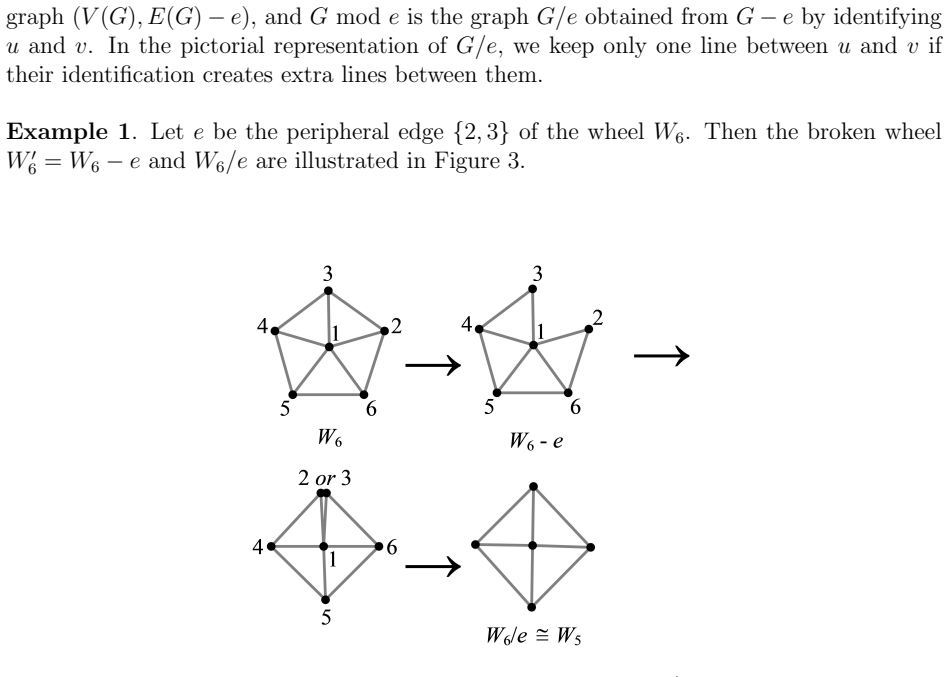
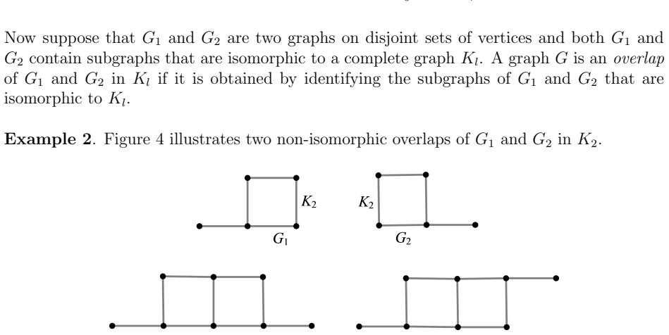
The machinery is the chromatic polynomial $\chi(G,t)$, combined with CRT-1 (overlap in a complete graph: $\chi(G,t)=\chi(G_1,t)\chi(G_2,t)/\chi(K_l,t)$) and CRT-2 (deletion-contraction: $\chi(G,t)=\chi(G-e,t)-\chi(G/e,t)$). The new object is the interlocking wheel $W_m\wedge_2 W_n$, two wheels identified along a two-vertex wedge; the Main Theorem formula expresses its chromatic polynomial in terms of wheel polynomials, letting the authors decompose large geographic graphs into pieces small enough for computer algebra.
What would settle it
Compute $\chi(W_6\wedge_2 W_7,4)$ directly with an independent deletion-contraction routine and compare it with the Main Theorem formula; if they differ, the interlocking-wheel formula and the France and USA counts are unsupported. Also rerun the paper's two decompositions of $G_A$ in a computer algebra system and compare the two reported values, 12,811,729,152 and 12,811,591,729,152.
Extended reading notes
Core claim
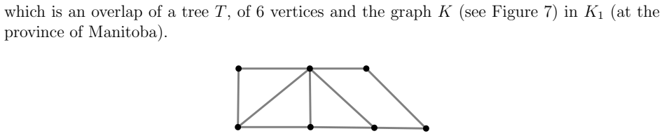
The authors claim that the chromatic polynomials of the Canada, France, and USA map graphs can be assembled from paths, cycles, complete graphs, and interlocking wheels using two reduction rules—deletion-contraction and overlap division—and that evaluating these polynomials at the appropriate number of colors gives the counts. The Main Theorem states a closed formula for $\chi(W_m\wedge_2 W_n,t)$, the chromatic polynomial of two wheels that share a two-vertex wedge, and this formula is what makes France and the USA computations feasible. For the USA the paper gives two values, 12,811,729,152 and 12,811,591,729,152, asserting both as the number of proper colorings from a four-color palette.
Load-bearing premise
The calculation assumes that two large algebraic expressions, which the paper says a computer program showed to be equal, really are equal; the paper shows no program code or output to verify this, and the two USA counts reported later disagree.
Editorial extensions
If this is right
- If the Main Theorem is correct, the number of proper four-colorings of the lower 48 states is either 12,811,729,152 or 12,811,591,729,152 depending on which of the paper's two decompositions is trusted, and including Alaska and Hawaii multiplies the count by 16.
- The count for the twelve contiguous regions of France is 5,184, and Canada's three-color count is 576.
- The Main Theorem extends the known wheel chromatic-polynomial formula to pairwise wedge-overlapping wheels, so other country maps containing interlocking wheels can be treated by the same reduction.
- The computed USA polynomial satisfies the paper's listed necessary conditions: it is monic of degree 48, has $t^{47}$ coefficient $-105$, has alternating signs, has zero constant term, and has coefficients summing to zero.
Reading between the lines
- The two reported USA values differ by roughly a factor of a thousand, so at most one can be right; an independent rerun of either 48-vertex decomposition in a symbolic computer system would settle the count.
- The Main Theorem's induction adds one wheel at a time, so the formula likely extends to chains of more than two interlocking wheels; testing a three-wheel chain would be a natural check.
- The same deletion-contraction plus overlap-division recipe could produce chromatic polynomials for other real maps whose graphs contain interlocking wheels, such as Mexico, Brazil, or Germany's Länder.
Signed reviews
Editorial analysis
A structured set of objections, weighed in public.
Referee Report
Summary. The paper computes chromatic polynomials of real geographic maps: Canada (576 three-colorings), metropolitan France (5184 four-colorings), and the contiguous United States. The USA computation is performed twice via deletion-contraction and CRT-1 decompositions of the 48-state graph G_A, and the paper presents a Main Theorem giving chi(W_m ^2 W_n, t) for interlocking wheels, used in the France and USA calculations. The paper's central claim is a single integer for the number of proper 4-colorings of the lower-48 map.
Significance. If correct, the Main Theorem would be a useful addition to the chromatic-polynomial toolbox for planar graphs containing interlocking wheels, and the Canada/France counts are natural data points not previously found in the literature. The paper uses only standard deletion-contraction identities and contains no fitted parameters, and it honestly describes the computational difficulties. However, the central USA count is given as two different integers with no reconciliation, and the crucial algebraic identities in the Main Theorem proof are asserted without machine-checkable support. As it stands, the headline result is not established.
major comments (3)
- [§6.3 and §7] The paper gives two different values for chi(G_A,4): in §6.3 (first attempt) it states 12,811,729,152, and in §7 (second attempt) it states 12,811,591,729,152. The second value is roughly 1000 times the first, and the text never acknowledges or reconciles the difference. Since the paper's central claim is a single integer for the number of proper 4-colorings of the lower-48 map, this internal contradiction means the main result is not established as written.
- [§5, Main Theorem proof] The two induction leaps in the proof of equation (3) are justified only by 'By Wolfram Mathematica e1-u2212e2 = 0', with no code, notebook, output, or independent algebraic derivation provided. These identities are load-bearing: formula (3) is used directly in the France computation and indirectly in the USA computations. Without a checkable verification, the Main Theorem and all subsequent counts rest on an unsupported assertion.
- [§6.3 and §7, second attempt] The second USA computation relies on Mathematica's evaluation of chi(X,t) for a 41-vertex, 93-edge graph X, but no code, output, or repoducible data are given for this step. Combined with the First Attempt, the reader has no way to verify either the decomposition into X and P or the final integers, and the claimed equality of the two attempts is not demonstrated.
minor comments (6)
- [§2] In the definition of P_2(V), the word 'carnality' should be 'cardinality'.
- [§5, proof of Theorem 3] The displayed expression 't(t−n)^{n−1}' appears to be a typographical corruption of t(t−1)^n; the intended algebra is clear from context but should be corrected.
- [§6.2, France polynomial] The final term of the displayed chromatic polynomial for G_F is '−3696y', which should be '−3696t'.
- [§6.3] In the footnote for the US map, 'Retrived' should be 'Retrieved'.
- [§5, Main Theorem base case] In the n=m=5 base case, the notation 'χ((W5∧2W5)+e,t)' is confusing because it does not name the graph before edge addition; the paragraph should define G=(W5∧2W5)−e explicitly before applying CRT-2.
- [§5, proof of Theorem 5] The sentence 'Let n≥3 be any integer such that it is true for all graphs with n≥3' is misworded; the intended inductive hypothesis is that the claim holds for all graphs on n vertices.
Circularity Check
No circularity: the paper's counts derive from deletion-contraction and CRT-1/CRT-2; the two divergent USA values and unverified Mathematica steps are correctness risks, not circular reductions.
full rationale
The paper's derivation chain is self-contained. Section 5 proves the wheel and cycle chromatic polynomials from the two Chromatic Reduction Theorems, and Section 6 applies these identities to geographic graphs. The Main Theorem for interlocking wheels is proved by double induction; the only questionable step is the invocation 'By Wolfram Mathematica e1−e2 = 0' in the induction, but that is an unsupported computational assertion, not a self-referential definition, a fitted input renamed as a prediction, or a result imported from the authors' own prior work. No parameter is fitted, no load-bearing self-citation occurs, and no equation in the paper defines its target in terms of itself. The internal inconsistency in Section 7—where χ(GA,4) is first reported as 12,811,729,152 and later as 12,811,591,729,152—is a genuine correctness failure in the central claim, as is the lack of verifiable evidence for the Mathematica equalities. However, under the stated rules, correctness gaps and unsupported computations are not circularity. Therefore the appropriate circularity score is 0.
Assumptions & free parameters
assumptions (3)
- standard math Chromatic Reduction Theorems (CRT-1 and CRT-2)
- ad hoc to paper Mathematica's polynomial simplifications are correct
- domain assumption Map graphs match geographic adjacencies
Cite this review
Pith. "Pith review of How many ways to color the map of America?." pith.science (2026). https://pith.science/paper/3HOVDBRR
@misc{pith2026190805694,
  author       = {Pith},
  title        = {Pith review of: How many ways to color the map of America?},
  year         = {2026},
  howpublished = {\url{https://pith.science/paper/3HOVDBRR}},
  note         = {Machine review of arXiv:1908.05694}
}
read the original abstract
Although the Four Color Conjecture originated in cartography, surprisingly, there is nothing in the literature on the number of ways to color an actual geographic map with four or fewer colors. In this paper, we compute these numbers, with exponentially increasing order of difficulty, for the maps of Canada, France, and the USA. Our attempts to compute the latter two lead to some new results on the chromatic polynomial of graphs.
Figures


Figures from the paper (15 more)




Reference graph
Works this paper leans on
-
[1]
Harary, Combinatorics, Addison-Wesley (1969)
F. Harary, Combinatorics, Addison-Wesley (1969)
work page 1969
-
[2]
Read, An Introduction to Chromatic Polynomials , J
R.C. Read, An Introduction to Chromatic Polynomials , J. Combinatorial Theory, 4(1968), 52–71. 22
work page 1968
Reviewed August 14, 2026 · model on record in the stance chip above.
Discussion (0). Continue with ORCID to comment.