REVIEW 4 major objections 6 minor 29 references
Physics-informed conditional diffusion model for generalizable elastic wave-mode separation
T0 review · 4 major / 6 minor · reviewed 2026-08-06 · deepseek-v4-flash
Pith's one-line read The paper claims that a single physics-informed conditional diffusion model, trained once, can separate elastic wave modes as accurately as conventional numerical solvers but at much lower cost, and that this one training run generalizes…
desk verdict A plausible new diffusion-based P/S separation method whose own 18 Hz failure contradicts the central claim that it learned the frequency-independent separation operator. read the letter →
The pith
A machine-rendered reading of the paper's core claim, the machinery that carries it, and where it could break.
The reading
What carries the argument
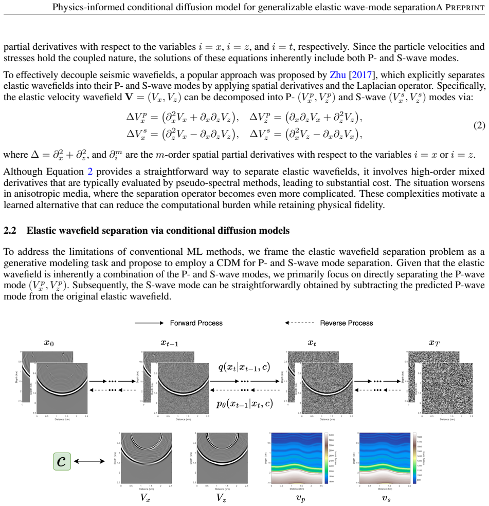
The load-bearing identity is the Laplacian separation system of Equation 2, which expresses the Laplacian of each P-wave velocity component as mixed second derivatives of the original elastic wavefield, for example $\Delta V^p_x = \partial^2_x V_x + \partial_x \partial_z V_z$, with no explicit velocity dependence. The model is an x0-prediction conditional diffusion U-Net that estimates the clean P-wave mode directly, and the physics enters in two places: as the training loss $\mathcal{L}_{\mathrm{phys}}$ enforcing exactly those Laplacian identities, and as a per-step sampling correction $\hat{x}_{t-1} \leftarrow \hat{x}_{t-1} - \eta \nabla \mathcal{L}_{\mathrm{phys}}$ during reverse diffusion, which steers the DDIM trajectory toward separation-consistent wavefields. This combination is what lets the inference run in as few as 10 reverse steps and is credited for the generalization across unseen models.
What would settle it
Generate an elastic wavefield with a source frequency outside the training band, for example a 15 Hz Ricker wavelet on the same SEAM Arid model, run the trained PICDM, and compare the predicted P-wave mode against the numerical reference of Equation 2: the paper's claim predicts a close match, whereas significant leakage or artifacts would show the model leaned on training-distribution cues. The paper's own 18 Hz experiment already fails in this way, which bounds the claim to the training-frequency band unless multi-frequency training is added.
Extended reading notes
Core claim
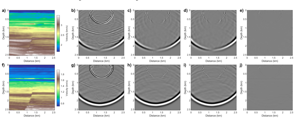
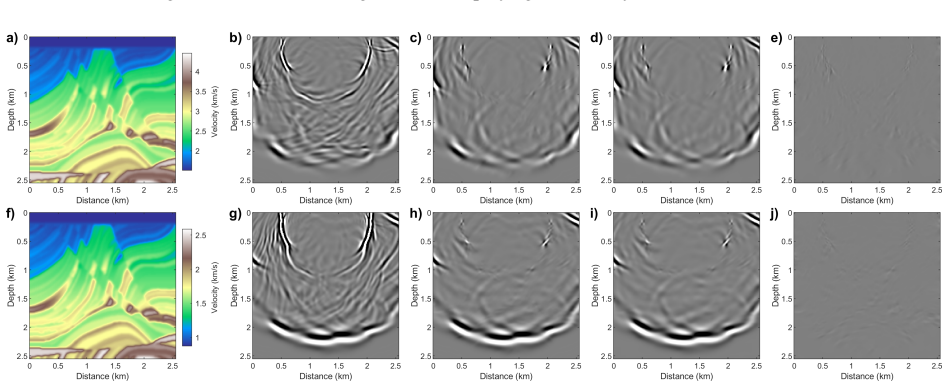
The central claim is that a single physics-informed conditional diffusion model (PICDM), trained once, can replace the numerical evaluation of the separation operator in Equation 2: conditioned on the elastic wavefield $(V_x, V_z)$ and the P- and S-wave velocity models, it outputs the clean P-wave mode $(\hat{V}^p_x, \hat{V}^p_z)$, and the S-wave mode is obtained by subtraction. In tests on a homogeneous medium, SEAM Arid, Overthrust, Marmousi 2, and Otway velocity models, on a larger $300 \times 640$ grid, and on a snapshot at 2.0 s (beyond the 1.5 s training window), the predicted P-wave modes closely match the conventional numerical solutions. The authors interpret this as the network internalizing the separation operator rather than memorizing training cases, since Equation 2 contains no explicit velocity-dependent terms; their ablation shows that removing velocity conditioning keeps in-distribution accuracy but degrades out-of-distribution separation, while an untrained source frequency of 18 Hz breaks the model entirely.
Load-bearing premise
The generalization claim rests on the assumption that during training the network internalized the actual separation operator rather than patterns tied to the 12 Hz source, the 10 m grid spacing, the constant density, the 0.52 to 0.7 $v_p/v_s$ scaling, and the 1.5 s simulation window, so that it will keep separating correctly when those quantities change.
Editorial extensions
If this is right
- Wave-mode separation for large or 3D surveys could run at the cost of a few DDIM steps instead of pseudo-spectral operator evaluations, making high-resolution imaging pipelines substantially cheaper.
- The model can be applied to geological models it has never seen, including faulted structures and realistic heterogeneous velocity distributions, without retraining or fine-tuning.
- Since the S-wave mode is computed by subtracting the predicted P-wave mode from the elastic wavefield, a single pass yields both modes in a mutually consistent way.
- Physics-guided sampling keeps separation quality stable with as few as 10 reverse steps, reducing inference time enough for interactive or high-throughput workflows.
- The demonstrated temporal extrapolation to a 2.0 s snapshot suggests the trained operator generalizes beyond the training window, though the 4.0 s failure bounds that reach.
Reading between the lines
- The 18 Hz failure is a built-in test of the learned-operator story, because Equation 2 contains no frequency terms; training on multi-peak-frequency data would both test and likely extend the model's envelope.
- The same recipe, conditioning a diffusion model on a known constraint and correcting samples by gradient backpropagation of that constraint, could be applied to other expensive wavefield operators such as up/down-going decomposition or attenuation compensation.
- Because the velocity-free ablation degrades only out of distribution, the velocity inputs may function as a contextual key that aligns wavefields and velocity structures with the training manifold; testing on $v_p/v_s$ ratios outside the 0.52 to 0.7 range would clarify whether the network truly learned an operator or a conditional lookup.
- The bounded temporal extrapolation (success at 2.0 s, artifacts at 4.0 s) suggests the generalization envelope is set by the variety of wavefront complexity in the training window, so longer simulations or more snapshots per model are a concrete path to widening it.
Editorial analysis
A structured set of objections, weighed in public.
Referee Report
Summary. The paper proposes a physics-informed conditional diffusion model (PICDM) for separating P-wave modes from elastic wavefields in 2D isotropic media. The method trains an x0-prediction diffusion model conditioned on the full elastic wavefield components and P/S velocity models, with a training loss that combines an ℓ2 data term and a physics-informed term based on the Laplacian separation equations of Zhu (2017). At inference, the same physics loss is used as a gradient-based correction during DDIM sampling. The authors evaluate the model on homogeneous media, SEAM Arid, Overthrust, Marmousi 2, Otway, a larger 300×640 model, and temporal extrapolation, and they include ablations without velocity conditioning and with an 18 Hz source. The paper claims that a single trained model achieves near-perfect agreement with numerical references across all these scenarios and that the model has effectively learned the frequency-independent separation operator of Eq. (2).
Significance. If the central claims hold, the contribution is potentially useful: a single diffusion model that replaces costly pseudo-spectral separation and generalizes across velocity models, model sizes, and time windows would be a practical advance, and the idea of embedding physics both in training and sampling is appealing. The paper also deserves credit for using a standard diffusion formulation, building on an open-source architecture, providing an ablation of velocity conditioning, and honestly disclosing the 18 Hz failure. However, the current evidence does not support the strongest claims: there are no quantitative error metrics or baseline comparisons, and the 18 Hz result directly contradicts the proposed operator-learning mechanism. The work is promising but needs substantial revision before the claims can be accepted.
major comments (4)
- [Section 4, Figure 16] The claim that the model 'has effectively learned the underlying separation operator described in Equation 2' is directly contradicted by the 18 Hz experiment. Equation 2 is a purely spatial differential relation with no dependence on source frequency, so a model that had internalized this operator should separate an 18 Hz wavefield as accurately as a 12 Hz one. The complete failure shown in Figure 16 indicates instead that the learned mapping is tied to the 12 Hz training distribution. This undermines the mechanism proposed in support of the 'learn once, apply everywhere' paradigm. Please either revise the mechanism claim or train with multi-frequency data and demonstrate that the operator-level generalization actually holds.
- [Sections 3.2–3.7 and Section 5] The central quantitative claims of 'almost perfectly match', 'near-perfect agreement', and 'minimal residual discrepancies' are supported only by qualitative residual images. No numerical error metrics (e.g., MSE, SNR, or normalized error) are reported for any test case, no error bars or repeated-run statistics are given, and no comparison is made against the existing learned baselines cited in the introduction (e.g., Wang and Ma 2019; Kaur et al. 2021; Meng et al. 2025). Please report per-experiment accuracy metrics, state the color scale values used in the residual plots, and benchmark against at least one prior learned separation method.
- [Sections 2.3–2.4, Eqs. (8)–(11)] The physics loss is not an independent check of physical consistency. The training labels are generated by the same Equation 2 that defines Lphys, so Ldata and Lphys are correlated by construction. More importantly, Equation 9 constrains only the Laplacian of the predicted P-wave field, and many different fields share the same Laplacian; the inference correction in Equation 11 minimizes the same residual and therefore cannot by itself select the correct P-wave field. The actual selection is performed by the data-driven prior learned from the training distribution. Please analyze this non-uniqueness explicitly and clarify what the physics term adds beyond a regularizer.
- [Section 3.7, Figures 12–13] The temporal extrapolation claim should be qualified quantitatively. The paper states that the method 'continues to accurately recover' the P-wave mode at 2.0 s but shows visible artifacts at 4.0 s; without error metrics it is unclear where the reliable extrapolation limit lies and how this relates to the 1.5 s training window. Please provide a time-sweep error curve or otherwise specify the maximum reliable extrapolation time supported by the data.
minor comments (6)
- [Section 3.1] The framework is referred to as 'PIGDM' in the opening of Section 3.1; this appears to be a typo for 'PICDM' and should be corrected.
- [Section 3.3] In the description of Figure 6, the text says 'following the same panel layout as in Figure 6' when it should refer to Figure 5; the panel layouts of the two figures differ because Figure 6 omits the velocity-model panels.
- [Section 3.2 and Figure 4] The accuracy metric in Figure 4 is described as MSE, but the y-axis labels and units are not provided, and no numerical values are quoted in the text; please add axis labels and state the numerical ranges.
- [Sections 2.4 and 3.1] The hyperparameters λ in Eq. (10) and η in Eq. (11) are never specified, and no sensitivity analysis is reported; please provide their values and, if possible, a brief sensitivity study.
- [Abstract and Section 3.3] The claim of 'reduced cost' is not supported by any wall-clock comparisons; please provide inference-time measurements against the numerical reference solver for at least the larger test cases.
- [Section 7] The code repository is currently private; to facilitate review, please provide an anonymized copy or specify a concrete release date.
Circularity Check
Central derivation is self-contained; only the physics-loss demonstration is tautological because Eq. 11 directly minimizes Eq. 9, while the 18 Hz failure is a generalization limitation, not circularity.
-
self definitional
[Section 2.4, Eq. (11); Figure 3; Section 3.2]
"The intermediate wavefield may still violate Equation (2). Therefore, we further apply a physics-guided correction to the intermediate prediction ˆxt−1 = (Vˆ p x , Vˆ p z ) by evaluating the physics-informed loss Lphys (e.g., Equation 9) and backpropagating its gradient: (Vˆ p x , Vˆ p z ) ← (Vˆ p x , Vˆ p z ) − η ∇Lphys. ... We can find that the diffusion model with physics guidance converges to a very low physical residual in far fewer steps."
Equation 11 is a gradient-descent step on Lphys, so the reduction in Lphys during physics-guided sampling (Figure 3) is true by construction; it shows the optimizer minimizing its own objective, not an independent check that the model has learned physics. Moreover, Lphys (Eq. 9) is the residual form of the same Zhu 2017 Laplacian operator (Eq. 2) used to generate the training labels, so the physics constraint and the reference solution are not fully independent. The main accuracy claim, however, is measured as MSE against the numerical reference on held-out wavefields, which is an external benchmark, so the central generalization result does not reduce to this loss.
full rationale
The paper's central claim—a single trained PICDM separates P-wave modes on in-distribution, out-of-distribution, larger, and temporally extrapolated models without retraining—is supported by held-out comparisons against numerical reference solutions obtained with Zhu's method. Those comparisons are legitimate supervised benchmarks, and no parameter is fitted to the test cases. The physics-informed loss (Eq. 9) and inference correction (Eq. 11) restate the same Laplacian separation operator (Eq. 2) that generates the labels; this is a standard physics-informed setup, but it means the physical-loss plots are a definitional consequence of the algorithm rather than independent evidence. That is a minor circularity in a supporting metric, not in the derivation itself. The paper's admitted 18 Hz failure (Figure 16) and the velocity-free ablation (Figures 14-15) undercut the speculation that the model 'has effectively learned the underlying separation operator' in a frequency- and velocity-independent sense, but these are generalization limitations honestly disclosed by the authors, not circular reasoning. The self-citations (SeparationPINN, Cheng et al. 2025) are motivational or analogical and do not carry the argument.
Assumptions & free parameters
free parameters (4)
- lambda (physics loss weight, Eq. 10) =
not reported
- eta (physics correction step size, Eq. 11) =
not reported
- DDIM sampling steps =
10
- S-wave velocity scaling range =
0.52 to 0.7 of vp
assumptions (5)
- domain assumption Zhu 2017 Laplacian equations (Eq. 2) define the correct P-wave mode and provide accurate training labels.
- domain assumption The first-order velocity-stress equations (Eq. 1) and the 10th-order finite-difference scheme produce physically accurate training wavefields.
- standard math The x0-prediction diffusion model with DDIM sampling approximates samples from the target conditional distribution.
- domain assumption A network trained on 150k examples from 6000 velocity models generalizes to unseen velocity models, larger grids, and later times.
- domain assumption Constant density, fixed 12 Hz source, and vp/vs derived by scalar multiplication are representative of the target application.
Cite this review
Pith. "Pith review of Physics-informed conditional diffusion model for generalizable elastic wave-mode separation." pith.science (2026). https://pith.science/paper/3JWNWQGG
@misc{pith2026250623007,
  author       = {Pith},
  title        = {Pith review of: Physics-informed conditional diffusion model for generalizable elastic wave-mode separation},
  year         = {2026},
  howpublished = {\url{https://pith.science/paper/3JWNWQGG}},
  note         = {Machine review of arXiv:2506.23007}
}
read the original abstract
Traditional elastic wavefield separation methods, while accurate, often demand substantial computational resources, especially for large geological models or 3D scenarios. Purely data-driven neural network approaches can be more efficient, but may fail to generalize and maintain physical consistency due to the absence of explicit physical constraints. Here, we propose a physics-informed conditional diffusion model for elastic wavefield separation that seamlessly integrates domain-specific physics equations into both the training and inference stages of the reverse diffusion process. Conditioned on full elastic wavefields and subsurface P- and S-wave velocity profiles, our method directly predicts clean P-wave modes while enforcing Laplacian separation constraints through physics-guided loss and sampling corrections. Numerical experiments on diverse scenarios yield the separation results that closely match conventional numerical solutions but at a reduced cost, confirming the effectiveness and generalizability of our approach.
Figures


Figures from the paper (13 more)





Reference graph
Works this paper leans on
-
[1]
2d and 3d elastic wavefield vector decomposition in the wavenumber domain for vti media
Qunshan Zhang and George A McMechan. 2d and 3d elastic wavefield vector decomposition in the wavenumber domain for vti media. Geophysics, 75 0 (3): 0 D13--D26, 2010
work page 2010
-
[2]
Jiubing Cheng and Sergey Fomel. Fast algorithms for elastic-wave-mode separation and vector decomposition using low-rank approximation for anisotropic media. Geophysics, 79 0 (4): 0 C97--C110, 2014
work page 2014
-
[3]
Keiiti Aki and Paul G Richards. Quantitative seismology. 2002
work page 2002
-
[4]
Elastic wave-mode separation for vti media
Jia Yan and Paul Sava. Elastic wave-mode separation for vti media. Geophysics, 74 0 (5): 0 WB19--WB32, 2009
work page 2009
-
[5]
Wave-field separation in two-dimensional anisotropic media
J Dellinger and J Etgen. Wave-field separation in two-dimensional anisotropic media. Geophysics, 55 0 (7): 0 914--919, 1990
work page 1990
-
[6]
Jia Yan and Paul Sava. Improving the efficiency of elastic wave-mode separation for heterogeneous tilted transverse isotropic media. Geophysics, 76 0 (4): 0 T65--T78, 2011
work page 2011
-
[7]
Jiubing Cheng, Tariq Alkhalifah, Zedong Wu, Peng Zou, and Chenlong Wang. Simulating propagation of decoupled elastic waves using low-rank approximate mixed-domain integral operators for anisotropic media. Geophysics, 81 0 (2): 0 T63--T77, 2016
work page 2016
-
[8]
Elastic wavefield separation based on the helmholtz decomposition
Hejun Zhu. Elastic wavefield separation based on the helmholtz decomposition. Geophysics, 82 0 (2): 0 S173--S183, 2017
work page 2017
Show all 29 references
-
[9]
Elastic wavefield separation in anisotropic media based on eigenform analysis and its application in reverse-time migration
Jidong Yang, Houzhu Zhang, Yang Zhao, and Hejun Zhu. Elastic wavefield separation in anisotropic media based on eigenform analysis and its application in reverse-time migration. Geophysical Journal International, 217 0 (2): 0 1290--1313, 2019
2019
-
[10]
Attenuation-compensated viscoelastic reverse time migration with finite difference operators
Xinru Mu, Tariq Alkhalifah, and Jianping Huang. Attenuation-compensated viscoelastic reverse time migration with finite difference operators. Geophysics, 90 0 (3): 0 1--53, 2024
2024
-
[11]
Ps decomposition of isotropic elastic wavefields using cnn-learned filters
W Wang and J Ma. Ps decomposition of isotropic elastic wavefields using cnn-learned filters. In 81st EAGE Conference and Exhibition 2019, volume 2019, pages 1--5. European Association of Geoscientists & Engineers, 2019
2019
-
[12]
A fast algorithm for elastic wave-mode separation using deep learning with generative adversarial networks (gans)
Harpreet Kaur, Sergey Fomel, and Nam Pham. A fast algorithm for elastic wave-mode separation using deep learning with generative adversarial networks (gans). Journal of Geophysical Research: Solid Earth, 126 0 (9): 0 e2020JB021123, 2021
2021
-
[13]
Deep learning-based p-and s-wave separation for multicomponent vertical seismic profiling
Yanwen Wei, Yunyue Elita Li, Jingjing Zong, Jizhong Yang, Haohuan Fu, and Mengyao Sun. Deep learning-based p-and s-wave separation for multicomponent vertical seismic profiling. IEEE Transactions on Geoscience and Remote Sensing, 60: 0 1--16, 2021
2021
-
[14]
P/s-wave separation of multicomponent seismic data at the land surface based on deep learning
He Huang, Tengfei Wang, and Jiubing Cheng. P/s-wave separation of multicomponent seismic data at the land surface based on deep learning. Geophysics, 88 0 (3): 0 V233--V247, 2023
2023
-
[15]
Up/down and p/s decomposition of distributed acoustic sensing-vertical seismic profiling data using multitask deep-learning method
Tao Meng, Tengfei Wang, Jiubing Cheng, Pengfei Duan, and Zhonglin Cao. Up/down and p/s decomposition of distributed acoustic sensing-vertical seismic profiling data using multitask deep-learning method. Geophysics, 90 0 (4): 0 V283--V296, 2025
2025
-
[16]
Separationpinn: Physics-informed neural networks for seismic p- and s-wave mode separation
Xinru Mu, Shijun Cheng, and Tariq Alkhalifah. Separationpinn: Physics-informed neural networks for seismic p- and s-wave mode separation. IEEE Transactions on Geoscience and Remote Sensing, pages 1--1, 2025
2025
-
[17]
Sh-wave propagation in heterogeneous media: Velocity-stress finite-difference method
Jean Virieux. Sh-wave propagation in heterogeneous media: Velocity-stress finite-difference method. Geophysics, 49 0 (11): 0 1933--1942, 1984
1933
-
[18]
P-sv wave propagation in heterogeneous media: Velocity-stress finite-difference method
Jean Virieux. P-sv wave propagation in heterogeneous media: Velocity-stress finite-difference method. Geophysics, 51 0 (4): 0 889--901, 1986
1986
-
[19]
Denoising diffusion probabilistic models
Jonathan Ho, Ajay Jain, and Pieter Abbeel. Denoising diffusion probabilistic models. Advances in neural information processing systems, 33: 0 6840--6851, 2020
2020
-
[20]
Improved denoising diffusion probabilistic models
Alexander Quinn Nichol and Prafulla Dhariwal. Improved denoising diffusion probabilistic models. In International conference on machine learning, pages 8162--8171. PMLR, 2021
2021
-
[21]
The 2004 bp velocity benchmark
FJ Billette and Sverre Brandsberg-Dahl. The 2004 bp velocity benchmark. In 67th EAGE Conference & Exhibition, pages cp--1. European Association of Geoscientists & Engineers, 2005
2004
-
[22]
3-d salt and overthrust seismic models
Fred Aminzadeh. 3-d salt and overthrust seismic models. 1996
1996
-
[23]
Survey design and implementation of a multiple wide-azimuth towed streamer seismic acquisition strategy at the tiber discovery; deep water gulf of mexico, usa
John C Naranjo, Eric J Ekstrand, John Etgen, Kenneth L Hargrove, James G Brewton, Oswaldo Garcia, Georgiy Astvatsaturov, Damian Hite, Bill Howieson, Bing Bai, et al. Survey design and implementation of a multiple wide-azimuth towed streamer seismic acquisition strategy at the ...
2011
-
[24]
Application of the perfectly matched absorbing layer model to the linear elastodynamic problem in anisotropic heterogeneous media
Francis Collino and Chrysoula Tsogka. Application of the perfectly matched absorbing layer model to the linear elastodynamic problem in anisotropic heterogeneous media. Geophysics, 66 0 (1): 0 294--307, 2001
2001
-
[25]
Decoupled weight decay regularization
Ilya Loshchilov and Frank Hutter. Decoupled weight decay regularization. arXiv preprint arXiv:1711.05101, 2017
2017 arXiv
-
[26]
Denoising diffusion implicit models
Jiaming Song, Chenlin Meng, and Stefano Ermon. Denoising diffusion implicit models. arXiv preprint arXiv:2010.02502, 2020
2010 arXiv
-
[27]
Seam update: The arid model—seismic exploration in desert terrains
Michael Oristaglio. Seam update: The arid model—seismic exploration in desert terrains. The Leading Edge, 34 0 (4): 0 466--468, 2015
2015
-
[28]
Marmousi2: An elastic upgrade for marmousi
Gary S Martin, Robert Wiley, and Kurt J Marfurt. Marmousi2: An elastic upgrade for marmousi. The leading edge, 25 0 (2): 0 156--166, 2006
2006
-
[29]
Seismic wavefield solutions via physics-guided generative neural operator
Shijun Cheng, Mohammad H Taufik, and Tariq Alkhalifah. Seismic wavefield solutions via physics-guided generative neural operator. arXiv preprint arXiv:2503.06488, 2025
2025 arXiv
Reviewed August 6, 2026 · model on record in the stance chip above.
Discussion (0). Continue with ORCID to comment.