REVIEW 6 minor 39 references
Stable spline identification of linear systems under missing data
T0 review · 0 major / 6 minor · reviewed 2026-08-14 · deepseek-v4-flash
Pith's one-line read This paper establishes that stable spline kernels induce a new family of radial basis function kernels describing filtered white noise, so missing output data can be imputed in closed form and the resulting models can outperform full-data…
desk verdict Solid extension of stable spline identification to missing data; the kernel derivation is clean and the central claims hold, with a real but non-fatal caveat about the Gaussian approximation in the marginal likelihood. read the letter →
The pith
A machine-rendered reading of the paper's core claim, the machinery that carries it, and where it could break.
The reading
What carries the argument
The load-bearing object is the RBF kernel family defined by Eq. (13), $h(x) = \int_0^\infty K(y, y+|x|)\,dy$, obtained by integrating the stable spline kernel $K$ along the diagonal; it expresses the second-order statistics of the noise component $\xi$ as a function of time lag only. For $q=1$ it reduces to the Laplace kernel $h(x) = e^{-\beta|x|}/\beta$, and for $q=2$ to $h(x) = (3e^{-2\beta|x|} - e^{-3\beta|x|})/(18\beta)$. This kernel, together with the stable spline output kernel $P$, enters the minimum variance linear estimator (24) and the marginal-likelihood criterion (26), which is optimized over only two or four hyperparameters before all missing outputs are returned in closed form.
What would settle it
Run a Monte Carlo with an ARMAX system whose noise-path pole is much faster than the system's least-damped pole, so the shared-$\beta$ RBF kernel is misspecified; if the closed-form imputer's mean-squared error on missing outputs is not close to that of the best linear estimator computed with the true noise covariance, the shared-$\beta$ assumption is load-bearing. A simpler check is to estimate the residual autocovariance from a long simulation and compare its shape with Eq. (15).
Extended reading notes
Core claim
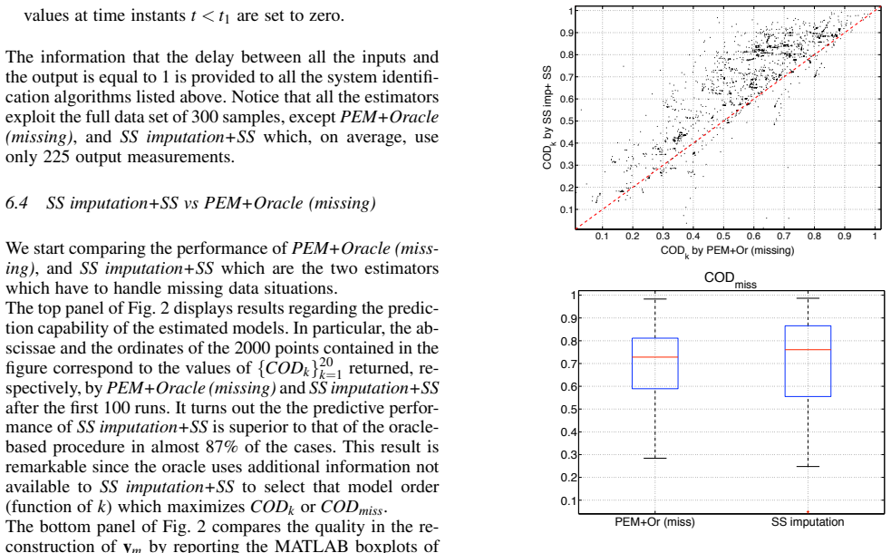
The central discovery is the covariance identity in Eq. (13): if the noise-path impulse response $f_p$ is a zero-mean Gaussian process with stable spline covariance $\lambda K$, then the disturbance $\xi(t) = (e \otimes f_p)(t)$ is a zero-mean stationary process whose covariance is the translation-invariant radial basis function $R(s,t) = h(s-t)$, where $h(x) = \int_0^\infty K(y, y+|x|)\,dy$. For the classic first- and second-order stable spline kernels this yields the explicit Laplace-like forms (14) and (15). Combined with the stable spline kernel for the system impulse responses, this makes the best linear predictor of the missing outputs in Eq. (24) computable in closed form; the paper calls the resulting procedure stable spline imputation. In Monte Carlo tests on ARMAX models with 25% output data missing, the imputation-then-identification pipeline produces models whose $k$-step-ahead prediction accuracy is better than that of PEM with oracle order selection in almost 87% of runs, and comparable to or better than full-data estimators.
Load-bearing premise
The estimator is the minimum variance linear one only when the disturbance process $\xi(t)$ is zero-mean stationary with covariance exactly $\lambda R$, which holds if the noise-path impulse response $f_p$ is drawn from a Gaussian process with stable spline covariance using the same stability decay $\beta$ as the system's impulse responses.
Editorial extensions
If this is right
- If the covariance identity holds, missing outputs can be imputed in closed form with no model-order search, just a two- or four-dimensional optimization for the hyperparameters.
- The estimator extends to continuous-time systems without re-derivation, since the kernel identities are stated for both discrete and continuous time.
- The approach can enrich the stable spline kernel with a low-order parametric component, so it can represent ARMAX systems with a small parametric part while retaining the closed-form imputer.
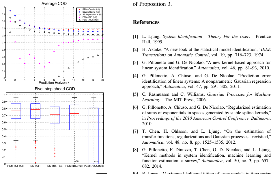
- In the experiments, imputation plus stable spline estimation matches or beats the full-data stable spline estimator and full-data PEM, suggesting that the imputed values do not degrade subsequent model quality.
- Because the estimate does not depend on the scale factor $\lambda$, imputation only requires relative hyperparameters, reducing the tuning burden.
Reading between the lines
- The covariance identity suggests a direct diagnostic: given a long record from a known system, the empirical autocorrelation of the residuals after removing the deterministic input could be compared against the predicted $h(x)$; a mismatch would indicate either a wrong $\beta$ or a noise path not well modeled by the stable spline prior.
- The same closed-form imputer could be adapted to missing inputs rather than outputs by symmetry of the linear model, though the paper only treats output gaps.
- Because the RBF kernel arises from a convolution, a similar construction may yield kernels for other Gaussian-process priors, such as Mat\'ern or periodic kernels, extending the family of tractable imputation problems.
Signed reviews
Editorial analysis
A structured set of objections, weighed in public.
Referee Report
Summary. The paper proposes a nonparametric Bayesian approach to identifying linear systems from output measurements with missing samples. The authors model the unknown impulse responses as zero-mean Gaussian processes with stable spline covariances and show that the disturbance component xi(t) = (e \otimes f_p)(t) is stationary with a covariance that is a new RBF kernel obtained by integrating the stable spline kernel along its diagonal (Proposition 1, Eq. (13), with discrete-time versions in Eqs. (17)-(19)). Using this kernel together with the stable spline kernel, they derive a closed-form linear minimum variance estimator for missing outputs (Proposition 3, Eq. (24)) and an algorithm, stable spline imputation (Algorithm 4), in which hyperparameters are estimated by marginal likelihood under a Gaussian approximation (Eq. (26)). Numerical experiments on ARMAX models compare the method against PEM baselines, including an oracle that selects model order on the test target, and report competitive or better predictive performance even when the benchmarks use the full data set.
Significance. If the results are correct, the paper makes a useful contribution to kernel-based system identification. The main theoretical content, the derivation of RBF kernels from stable spline priors, is transparent and checkable: the q=1 case reduces to the Laplace kernel, and the q=2 closed form is consistent with direct summation. The estimator in Proposition 3 is the standard linear minimum variance expression, and the independence structure of the Bayesian network is clearly specified. The experimental design is strong: the PEM baselines include oracle order selection on the test target, which gives the parametric competitors an advantage, and the conclusion that the nonparametric imputation method is competitive is carefully worded. The paper is also clearly organized, and its scope covers both discrete- and continuous-time settings, which is broader than most existing missing-data solutions. The acknowledged Gaussian approximation in the marginal likelihood is a limitation but not an internal inconsistency. Overall this is a solid, publishable contribution.
minor comments (6)
- [Section 2.3, Eqs. (6)-(7)] The notation for R_m is inconsistent: the text calls it a covariance matrix, but the displayed definition in Eq. (6) is E[\xi_m \xi^T], which is a cross-covariance, and Eq. (7) uses it in exactly that cross-covariance role. Please define R_{mo} = E[\xi_m \xi^T] explicitly and use a separate symbol for the auto-covariance of \xi_m, or state clearly that R_m denotes the cross-covariance.
- [Section 4.2, Proposition 1] The proof of Proposition 1 is omitted with the note that it relies on simple computations. Since this proposition is the main theoretical novelty of the paper, please include a derivation in the appendix; this would also clarify the integration over R_+ and the role of |x|.
- [Section 5.3, Eq. (26)] The Gaussian approximation for the disturbance is introduced but not discussed. Please add a sentence or two explaining the nature of the approximation and its expected effect on hyperparameter estimates; a brief empirical check would strengthen the paper, although the current experiments do not indicate a problem.
- [Section 6.5, bottom panel] The text says 'boxplots of the 1000 values of COD5' but the Monte Carlo study has 500 runs; this appears to be a typo and should be corrected to 500.
- [Section 6.4, top panel] The sentence reporting 'almost 87% of the cases' should clarify whether 'cases' refers to the 2000 individual COD_k values from the first 100 runs or to the number of Monte Carlo runs; the current wording is ambiguous.
- [Section 5.1, Eq. (21)] The definition of h_x(t) in the output kernel P(x,y) is hard to parse. Please rewrite it with a more explicit convolution formula, such as P(x,y) = \sum_l \int\int u_l(y-s) u_l(x-r) K(s,r) ds dr, or state clearly that h_x(t) is the function t \mapsto (u_l(\cdot) \otimes K(t,\cdot))(x).
Circularity Check
No significant circularity: the new RBF kernel class is derived from the stable spline prior, and the imputation estimator is a standard Bayesian/linear-minimum-variance construction with an acknowledged Gaussian approximation.
full rationale
I walked the paper's derivation chain. Proposition 1 (Eq. 13) computes the covariance of the disturbance xi(t) = (e ⊗ f_p)(t) by integrating the assumed stable spline covariance K(y, y+|x|) over y; the closed forms (14)-(15) in continuous time and (18)-(19) in discrete time follow by direct integration or summation from the stated q=1 and q=2 stable spline kernels. These are genuine derived quantities, not renamed inputs, and they match direct computation, providing an external check. The estimator in Proposition 3 (Eqs. 24-25) is the standard linear minimum variance estimator: V(y_o) = lambda(P+R) and the cross-covariance V(y(t), y_o) = lambda(P(t,·)+R(t,·)) follow from the stated mutual independence of e and the f_l's, with no fitted parameter secretly renamed as a prediction. Hyperparameter estimation via marginal likelihood (Eq. 26) uses only the observed vector y_o, while the imputation target y_m is not used to fit the hyperparameters; the Gaussian approximation for the disturbance is explicitly acknowledged in the text as an approximation, which is a modeling limitation rather than a circular step. The paper does cite the authors' prior stable spline framework, but that framework is used as the prior assumption from which the new RBF class is derived; the cited results do not contain the target RBF/imputation result, and the numerical comparisons against PEM baselines, including an oracle-order PEM that sees the full data, provide independent evidence for the performance claim. No equation in the paper reduces to its own inputs by construction, and no fitted quantity is presented as an independent prediction in a way that would constitute circularity.
Assumptions & free parameters
free parameters (3)
- β (stable spline decay) =
estimated from data via marginal likelihood (Eq. 26)
- λ (scale factor) =
estimated from data via marginal likelihood (Eq. 26)
- φ, ϕ (ARMAX pole parameters) =
estimated from data when the enriched kernel is used
assumptions (5)
- domain assumption Each impulse response f_l is a zero-mean Gaussian process with covariance λK_l, where K_l is the stable spline kernel (or its enriched version).
- domain assumption The innovation e is zero-mean white noise with unit variance and is independent of all f_l.
- domain assumption The disturbance ξ(t) = (e ⊗ f_p)(t) is a stationary process with finite second-order moments, and the convolution is well defined.
- ad hoc to paper The marginal likelihood for hyperparameter estimation is computed under a Gaussian approximation of the output distribution.
- domain assumption Missing output data are missing at random (MCAR).
Cite this review
Pith. "Pith review of Stable spline identification of linear systems under missing data." pith.science (2026). https://pith.science/paper/3N7X5TJS
@misc{pith2026190803913,
  author       = {Pith},
  title        = {Pith review of: Stable spline identification of linear systems under missing data},
  year         = {2026},
  howpublished = {\url{https://pith.science/paper/3N7X5TJS}},
  note         = {Machine review of arXiv:1908.03913}
}
read the original abstract
A different route to identification of time-invariant linear systems has been recently proposed which does not require committing to a specific parametric model structure. Impulse responses are described in a nonparametric Bayesian framework as zero-mean Gaussian processes. Their covariances are given by the so-called stable spline kernels encoding information on regularity and BIBO stability. In this paper, we demonstrate that these kernels also lead to a new family of radial basis functions kernels suitable to model system components subject to disturbances given by filtered white noise. This novel class, in cooperation with the stable spline kernels, paves the way to a new approach to solve missing data problems in both discrete and continuous-time settings. Numerical experiments show that the new technique may return models more predictive than those obtained by standard parametric Prediction Error Methods, also when these latter exploit the full data set.
Figures

Figures from the paper (1 more)
Reference graph
Works this paper leans on
-
[1]
Ljung, System Identification - Theory For the User
L. Ljung, System Identification - Theory For the User . Prentice Hall, 1999
work page 1999
-
[2]
A new look at the statistical model identification,
H. Akaike, “A new look at the statistical model identification,” IEEE Transactions on Automatic Control , vol. 19, pp. 716–723, 1974
work page 1974
-
[3]
A new kernel-based approach for linear system identification,
G. Pillonetto and G. De Nicolao, “A new kernel-based approach for linear system identification,” Automatica, vol. 46, pp. 81–93, 2010
work page 2010
-
[4]
Prediction error identification of linear systems: A nonparametric Gaussian regression approach,
G. Pillonetto, A. Chiuso, and G. De Nicolao, “Prediction error identification of linear systems: A nonparametric Gaussian regression approach,” Automatica, vol. 47, pp. 291–305, 2011
work page 2011
-
[5]
C. Rasmussen and C. Williams, Gaussian Processes for Machine Learning. The MIT Press, 2006
work page 2006
-
[6]
Regularized estimation of sums of exponentials in spaces generated by stable spline kernels,
G. Pillonetto, A. Chiuso, and G. De Nicolao, “Regularized estimation of sums of exponentials in spaces generated by stable spline kernels,” in Proceedings of the 2010 American Control Conference, Baltimora, 2010
work page 2010
-
[7]
On the estimation of transfer functions, regularizations and Gaussian processes - revisited,
T. Chen, H. Ohlsson, and L. Ljung, “On the estimation of transfer functions, regularizations and Gaussian processes - revisited,” Automatica, vol. 48, no. 8, pp. 1525–1535, 2012
work page 2012
-
[8]
Kernel methods in system identification, machine learning and function estimation: a survey,
G. Pillonetto, F. Dinuzzo, T. Chen, G. D. Nicolao, and L. Ljung, “Kernel methods in system identification, machine learning and function estimation: a survey,” Automatica, vol. 50, no. 3, pp. 657– 682, 2014
work page 2014
Show all 39 references
-
[9]
Maximum likelihood fitting of arma models to time series with observations,
R. Jones, “Maximum likelihood fitting of arma models to time series with observations,” Technometrics, vol. 22, pp. 389–395, 1980
1980
-
[10]
Exact likelihood of vector autoregressive- moving average process with missing or aggregated data,
C. F. Ansley and R. Kohn, “Exact likelihood of vector autoregressive- moving average process with missing or aggregated data,” Biometrika, vol. 70, no. 1, pp. 275–278, 1983
1983
-
[11]
The exact likelihood of an autoregressive- moving average model with incomplete data,
J. Penzer and B. Shea, “The exact likelihood of an autoregressive- moving average model with incomplete data,” Biometrika, vol. 84, no. 4, pp. 919–928
-
[12]
Autoregressive spectral analysis when observations are missing,
P. Broersen, S. de Waele, and R. Bos, “Autoregressive spectral analysis when observations are missing,” Automatica, vol. 40, pp. 1495–1504, 2004
2004
-
[13]
Gilks, S
W. Gilks, S. Richardson, and D. Spiegelhalter, Markov chain Monte Carlo in Practice . London: Chapman and Hall, 1996
1996
-
[14]
Estimation of time series models in the presence of missing data,
W. Dunsmuir and P. Robinson, “Estimation of time series models in the presence of missing data,” Journal of the American Statistical Association, vol. 76, pp. 560–568, 1981
1981
-
[15]
Frequency domain system identification with missing data,
R. Pintelon and J. Schoukens, “Frequency domain system identification with missing data,” IEEE Transactions on Automatic Control, vol. 45, pp. 364–369, 2000
2000
-
[16]
Maximum likelihood from incomplete data via the em algorithm,
A. P. Dempster, N. M. Laird, and D. B. Rubin, “Maximum likelihood from incomplete data via the em algorithm,” Journal of the Royal Statistical Society. Series B (Methodological) , vol. 39, no. 1, pp. 1–38, 1977. [Online]
1977
-
[17]
Identification of ARX models subject to missing data,
A. Isaksson, “Identification of ARX models subject to missing data,” IEEE Transactions on Automatic Control, vol. 38, pp. 813–819, 1993
1993
-
[18]
Soderstrom and P
T. Soderstrom and P. Stoica, System Identification . Prentice Hall, 1989
1989
-
[19]
A Bayesian learning approach to linear system identification with missing data,
G. Pillonetto and A. Chiuso, “A Bayesian learning approach to linear system identification with missing data,” in Proceedings of the 48th IEEE International Conference on Decision and Control , S. Mendelson and A. J. Smola, Eds., Shangai, China, 2009
2009
-
[20]
B. D. O. Anderson and J. B. Moore, Optimal Filtering. Englewood Cliffs, N.J., USA: Prentice-Hall, 1979. 9 0 5 10 15 200 0.1 0.2 0.3 0.4 0.5 0.6 0.7 0.8 0.9 1 Prediction Horizon k Average COD 0 5 10 15 200 0.1 0.2 0.3 0.4 0.5 0.6 0.7 0.8 0.9 1 Prediction Horizon k Average COD F...
1979
-
[21]
Wahba, Spline models for observational data
G. Wahba, Spline models for observational data . SIAM, Philadelphia, 1990
1990
-
[22]
Networks for approximation and learning,
T. Poggio and F. Girosi, “Networks for approximation and learning,” in Proceedings of the IEEE , vol. 78, 1990, pp. 1481–1497
1990
-
[23]
Regression and time series model selection in small samples,
C. Hurvich and C. Tsai, “Regression and time series model selection in small samples,” Biometrika, vol. 76, pp. 297–307, 1989
1989
-
[24]
Bisiacco and G
M. Bisiacco and G. Pillonetto. On the Mathematical foundations of stable RKHSs. Automatica, 2020
2020
-
[25]
Bisiacco and G
M. Bisiacco and G. Pillonetto. Kernel absolute summability is sufficient but not necessary for RKHS stability. SIAM Journal on Control and Optimization , 2020
2020
-
[26]
Bottegal, A.Y
G. Bottegal, A.Y . Aravkin, H. Hjalmarsson, and G. Pillonetto. Robust EM kernel-based methods for linear system identification. Automatica, 67:114 – 126, 2016
2016
-
[27]
T. Chen. On kernel design for regularized lti system identification. Automatica, 90:109 – 122, 2018
2018
-
[28]
T. Chen, M. S. Andersen, L. Ljung, A. Chiuso, and G. Pillonetto. System identification via sparse multiple kernel-based regularization using sequential convex optimization techniques. IEEE Transactons on Automatic Control , provisionally accepted, 2013
2013
-
[29]
T. Chen, L. Ljung, M. Andersen, A. Chiuso, F.P. Carli, and G. Pillonetto. Sparse multiple kernels for impulse response estimation with majorization minimization algorithms. In IEEE Conference on Decision and Control , pages 1500–1505, Hawaii, Dec 2012
2012
-
[30]
Chen and G
T. Chen and G. Pillonetto. On the stability of reproducing kernel Hilbert spaces of discrete-time impulse responses. Automatica, 95:529 – 533, 2018
2018
-
[31]
Chiuso, T
A. Chiuso, T. Chen, L. Ljung, and G. Pillonetto. Regularization strategies for nonparametric system identification. In Proceedings of the 52nd Annual Conference on Decision and Control (CDC) , 2013
2013
-
[32]
Darwish, G
M.A.H. Darwish, G. Pillonetto, and R. Toth. The quest for the right kernel in Bayesian impulse response identification: The use of obfs. Automatica, 87:318 – 329, 2018
2018
-
[33]
F. Dinuzzo. Kernels for linear time invariant system identification. SIAM Journal on Control and Optimization , 53(5):3299–3317, 2015
2015
-
[34]
Ljung, T
L. Ljung, T. Chen, and B. Mu. A shift in paradigm for system identification. International Journal of Control , pages 1–8, 2019
2019
-
[35]
Pillonetto
G. Pillonetto. Consistent identification of Wiener systems: A machine learning viewpoint. Automatica, 49(9):2704–2712, September 2013
2013
-
[36]
Pillonetto
G. Pillonetto. A new kernel-based approach to hybrid system identification. Automatica, 70:21 – 31, 2016
2016
-
[37]
Pillonetto
G. Pillonetto. System identification using kernel-based regularization: New insights on stability and consistency issues. Automatica, 93:321– 332, 2018
2018
-
[38]
Pillonetto, T
G. Pillonetto, T. Chen, A. Chiuso, G. De Nicolao, and L. Ljung. Regularized linear system identification using atomic, nuclear and kernel-based norms: The role of the stability constraint. Automatica, 69:137 – 149, 2016
2016
-
[39]
Pillonetto and A
G. Pillonetto and A. Chiuso. Tuning complexity in regularized kernel- based regression and linear system identification: The robustness of the marginal likelihood estimator. Automatica, 58:106 – 117, 2015. 10
2015
Reviewed August 14, 2026 · model on record in the stance chip above.
Discussion (0). Continue with ORCID to comment.