REVIEW 4 major objections 4 minor 89 references
Nonlinear Diffusion and Decay of an Expanding Turbulent Blob
T0 review · 4 major / 4 minor · reviewed 2026-08-07 · deepseek-v4-flash
Pith's one-line read An isolated turbulent blob in still water spreads and decays by a single nonlinear diffusion equation, with a sharp front advancing as (t-t0)^0.38 and a universal (t-t0)^-2 decay once the integral length scale saturates.
desk verdict This is a serious experimental paper whose expansion-phase result—a directly measured sharp front with 0.38 collapse exponent and a measured l(t) that kills the instantaneous-eddy-adaptation assumption—is new and convincing; the late-time modeling claim is not. read the letter →
The pith
A machine-rendered reading of the paper's core claim, the machinery that carries it, and where it could break.
The reading
What carries the argument
The carrying object is the Kolmogorov-Barenblatt turbulent energy balance equation, $$\partial_t q = \tfrac{2}{3} c_0 \ell(t) \$nabla^{2}$ $q^{{3/2}}$ - \varepsilon_0 \frac{$q^{{3/2}}$}{\ell(t)},$$ a porous-medium-type nonlinear diffusion equation for the turbulence energy density $q$. The superlinear transport term $\nabla^2 q^{3/2}$ (exponent $m = 3/2 > 1$) does the central work: unlike linear diffusion it yields compactly supported self-similar fronts with profile $q \propto [1-(r/h)^2]^2_+$ and a sharp cutoff at $r = h(t)$, so the turbulent-non-turbulent boundary propagates at finite speed instead of sending a Gaussian precursor. The measured integral length scale $\ell(t)$ enters both transport and dissipation, making it the single control parameter of the decay rate: constant $\ell$ forces $q \sim t^{-2}$, while a growing $\ell$ slows the decay. Supporting machinery includes the log-movie PIV acquisition (frame spacing grows so tracer displacement stays measurable while velocities drop by three orders of magnitude), the virtual-origin cross-validated power-law fit, and the Cell Dynamical System split-step solver that integrates the stiff, front-bearing equation from experimental initial conditions.
What would settle it
Follow the same isolated blob in a domain large enough that the eddies never feel the walls — a much larger tank, or a direct numerical simulation box with an identical initial blob — and check two predictions at once: the front profile should stay compact, $q \propto [1-(r/h)^2]^2_+$ with no exponential tail and $h \sim (t-t_0)^{0.38}$, and the decay exponent should change only when the measured $\ell(t)$ changes. An exponential front tail, or a decay-rate change uncorrelated with $\ell(t)$, would refute both the $m = 3/2$ nonlinearity and the claim that $\ell$ controls the decay exponent.
Extended reading notes
Core claim
On the paper's own terms, an ensemble-averaged, isolated decaying turbulent blob obeys $$\partial_t q = \tfrac{2}{3} c_0 \ell(t) \$nabla^{2}$ $q^{{3/2}}$ - \varepsilon_0 \frac{$q^{{3/2}}$}{\ell(t)},$$ with transport closure $\kappa_q = c_0 \ell \sqrt{q}$ and dissipation $\varepsilon = \varepsilon_0 q^{3/2}/\ell$ taken from Kolmogorov's similarity hypotheses, the integral length scale $\ell(t)$ measured from the three-dimensional energy spectrum, and $O(1)$ coefficients $c_0 \approx 1.2$, $\varepsilon_0 \approx 0.88$. The front measurement uses a smaller, more localized blob so propagation can be followed before walls are reached; the decay laws use a larger blob with initial $Re_\lambda = 203$. Three consequences are then verified: the turbulent-quiescent boundary is a sharp front with a compact profile that propagates non-diffusively as $r \sim (t-t_0)^{0.38}$ (predicted $0.389$); during free expansion the spatially averaged energy decays as $(t-t_0)^{-1.3}$ while $\ell(t) \sim t^{0.16}$ is still growing; and once $\ell$ saturates at roughly a quarter of the chamber width, decay becomes the universal $(t-t_0)^{-2}$, reproduced from the start in a control experiment with a double oscillating grid whose $\ell$ is constant. Throughout the 17 minutes, rescaling the energy spectra by the measured dissipation collapses them onto the universal dissipation-range profile down to $Re_\lambda \approx 10$, so the cascade's fingerprint survives into the final decay.
Load-bearing premise
The load-bearing premise is that the measured two-dimensional integral length scale $\ell(t)$ faithfully represents the three-dimensional eddy field and that the two Kolmogorov closures — transport $\kappa_q = c_0 \ell \sqrt{q}$ and dissipation $\varepsilon = \varepsilon_0 q^{3/2}/\ell$ — hold at every instant, down to $Re_\lambda \approx 10$ and across the moment the blob touches the tank walls; the paper itself drops $c_0$ from $1.2$ to $0.001$ after wall contact to reproduce the observed crossover, conceding that the closure fails in exactly that regime.
Editorial extensions
If this is right
- Decay-exponent scatter across grid, pipe, and spin-down experiments is explained as differences in how the integral length scale grows in each apparatus, with constant $\ell$ always yielding $t^{-2}$.
- Because the front is sharp and propagates at finite speed with no Gaussian precursor, an aircraft or probe crossing into a turbulent patch would encounter it abruptly; the model gives that invasion speed from local $q$ and $\ell$.
- Turbulent statistics remain on the universal dissipation-range spectrum down to $Re_\lambda \approx 10$, so flow that looks still to the eye can still be fully turbulent, and naked-eye quiescence is not a valid stopping criterion for decay experiments.
- The same $O(1)$ coefficients ($c_0 \approx 1.2$, $\varepsilon_0 \approx 0.88$) reproduce both the instantaneous front speed and the long-time decay curve, so the model is quantitative rather than merely scaling-consistent.
- Only the ensemble-averaged field obeys the mean-field equation; single realizations spread in a branched, non-uniform manner, so the equation's predictions are statistical statements about many realizations.
Reading between the lines
- The paper's own need to cut $c_0$ from $1.2$ to $0.001$ after wall contact points to what a next model should add: a second field for the chamber-filling circulation that wall interaction feeds, which would let the crossover time be predicted rather than fitted.
- If the sharp-front solution is as strong an attractor as the initial-condition tests suggest, the same equation should describe natural turbulent patches — island wakes, convective thermals, ash clouds — where the front's finite speed sets how fast a patch can contaminate surrounding quiescent fluid; field measurements of $q(r,t)$ and $\ell(t)$ would suffice to test it.
- The log-movie acquisition idea transfers to any power-law-dominated dynamics — gravity currents, phase separation, critical-point relaxation — as a way to span many decades of time in one recording with constant tracer displacement; applying it to a different self-similar system would be a direct check of its generality.
- A clean test of the $\ell$-governance claim: in a much larger chamber the $(t-t_0)^{-1.3}$ regime should persist longer and the crossover should occur exactly when $\ell$ saturates; a decay-exponent change while $\ell$ is still measurably growing would falsify it.
Editorial analysis
A structured set of objections, weighed in public.
Referee Report
Summary. The paper reports an experimental study of an isolated turbulent blob created by eight converging vortex rings in a water tank, with ensemble-averaged PIV measurements over several decades of time using a logarithmic sampling scheme. The central claim is that the spatiotemporal evolution of the blob is governed by the nonlinear diffusion equation Eq. (4), ∂t q = (2/3)c0 l ∇^2 q^{3/2} - ε0 q^{3/2}/l, with spatially uniform, measured integral length scale l(t). The authors present evidence for a sharp turbulent-quiescent front that propagates non-diffusively with self-similar collapse exponent ~0.38 (predicted 0.389), report agreement between the measured expansion rate Rdot and Eq. (4) with fitted coefficients c0=1.2 and ε0=0.88, and reproduce the late-time q~(t-t0)^-2 decay when l is constant. They also acknowledge that the fixed-closure simulation enters the q~(t-t0)^-2 regime earlier than the experiment and that reducing c0 to 0.001 is needed to delay the crossover, attributing the discrepancy to persistent eddy structures beyond the mean-field model.
Significance. The expansion-phase evidence, if taken alone, is a substantial contribution: the authors provide a controlled, boundary-free experimental configuration for studying turbulent-non-turbulent front propagation, and the sharp-front prediction, the non-diffusive propagation scaling, and the absence of Gaussian spreading are parameter-free qualitative consequences of the nonlinear transport term in Eq. (4). The log-movie acquisition method is a practical and broadly applicable technique for power-law decaying flows, and the cross-validation virtual-origin method is a useful analysis tool. The comparison across three different forcing methods in the same chamber, and the demonstration that a constant l gives q~(t-t0)^-2, strengthen the empirical part of the paper. However, the quantitative validation of Eq. (4) as a fixed-coefficient model is incomplete, because c0 and ε0 are fitted to data that are also used for validation, and because the crossover to the t^-2 regime is reproduced only after a three-order-of-magnitude change in c0 that is not derived from the model.
major comments (4)
- [Main text, Fig. 2c; SI §V.E] The paper's broad claim that Eq. (4) accounts for the detailed spatiotemporal decay is not supported by the fixed-coefficient model as stated. The blue CDS curve in Fig. 2c, computed with (c0, ε0)=(1.2, 0.88) and the measured l(t), enters the q~(t-t0)^-2 regime much earlier than the experiment. The cure, reducing c0 to 0.001, changes the transport coefficient by three orders of magnitude, and SI §V.E explicitly attributes the need to persistent eddy structures that are 'beyond the scope' of the mean-field model. Since the transport term in Eq. (4) is proportional to c0 and c0 is presented as a fixed dimensionless constant from Kolmogorov similarity, this is a regime dependence of the central closure rather than a routine parameter adjustment. The expansion-phase conclusions (Fig. 5) are largely independent of this issue, but the abstract and conclusion should be revised to state that Eq. (4) applies to the free-expansion phase and that the wall-filling crossover is captured only with an empirically modified c0, or an additional closure for the persistent inhomogeneity should be provided.
- [Eq. (1) and Fig. 4a-b] The validation of the dissipation relation is partially circular. The value ε0=0.88±0.10 is estimated from the asymptotic decay by solving dq/dt=-ε0 q^{3/2}/l_sat assuming q~(t-t0)^-2, and the same relation is then presented as 'agreement' in Fig. 4a. To establish Eq. (1) independently, ε0 should be estimated from a direct measurement such as the structure-function or strain-rate methods described in SI §IV.C.4, without using the decay curve itself, or the circularity should be explicitly acknowledged and its influence on the reported uncertainty quantified.
- [Eq. (4) and Table III] The model treats l(t) as a spatially uniform, exogeneous input and assumes the closures κq=c0 l sqrt(q) and ε=ε0 q^{3/2}/l hold for the ensemble-averaged 3D energy field down to Re_lambda~10 and across the wall-filling phase. The paper's own Fig. 2c shows the fixed closure fails in exactly the wall-filling regime, and SI §V.A reports persistent eddy structures that are not captured by the mean-field radial description. A clear statement of the regime of validity of Eq. (4) (free expansion, ensemble-averaged fields, and a lower Reynolds-number bound) is needed before the model can be claimed as a general framework for decaying turbulence.
- [Fig. 2c and SI Table III] The comparison between the fast-transport and slow-transport simulations is confounded by the use of different initial conditions and initial times. The main-text Fig. 2c caption states that the fast simulation uses the ensemble-averaged profile at t=0.4 s and the slow one uses t=2 s, while SI Table III lists t=0.5 s for the slow case. This discrepancy should be resolved, and the two simulations should be initialized from the same time and the same field, or the dependence of the crossover on the initial condition should be shown, so that the delayed crossover can be attributed specifically to the change in c0.
minor comments (4)
- [SI §IV.C.3] The virtual-origin fitting method is described briefly in the main text; please specify the number of cross-validation folds, the procedure for selecting the fitting window [ta,tb], and how the reported r^2 values account for the number of data points, since the exponential spacing of the logarithmic sampling makes the effective sample size window-dependent.
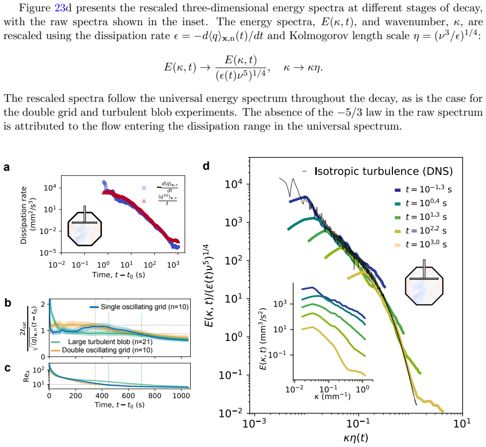
- [Main text, Fig. 4d and SI §IV.C.4] The statement that the energy spectra collapse onto a universal DNS profile should clarify whether the collapse is obtained by rescaling with the measured dissipation rate from -d<q>_x,n/dt or with a fitted dissipation rate, because the spectral and structure-function methods in SI yield different ε values at late times.
- [Main text, Eq. (3) and SI §II.B] The factor 2/3 appears in Eq. (4) but is not present in the SI radial equation (17); please clarify whether c0 in the SI is redefined or whether the factor arises from the identity ∇^2 q^{3/2} = (3/2) q^{1/2} ∇^2 q + (3/4) q^{-1/2} |∇q|^2, and state the convention consistently throughout.
- [Main text, Fig. 5b-c and SI §V.B] The error map in Fig. 5c shows a linear valley of near-minimal error, meaning that c0 and ε0 are not independently determined by the Rdot measurement. The paper should state explicitly that the quoted c0=1.2 relies on the independently chosen ε0=0.88, and that the Rdot data alone would allow a range of (c0, ε0) combinations.
Circularity Check
Two fitted inputs are presented as reproductions (ε0 from the late-time decay curve and (c0, ε0) from Ṙblob), but the parameter-free exponents (−2, 0.389, 0.51) and the paper's own c0 = 0.001 disclosure keep the core derivation from Eq. 4 self-contained.
-
fitted input called prediction
[Main text, parameters-estimation paragraph (p. 4) and Fig. 2c caption]
"ε0 can also be experimentally estimated using the late-time decay dynamics where q ∼ t−2 and ℓ remains constant at ℓsat. By solving dq/dt = −ε0 q3/2/ℓsat, we obtain ε0 = 2ℓsat/[√q(t−t0)] [...] (c) Using experimentally determined initial conditions and the integral length scale, the 3D cell dynamical systems simulations reproduce the observed power laws."
The late-time solution of the model with constant ℓ is q(t) = [2ℓsat/(ε0(t−t0))]², which is exactly the inverse of the defining relation ε0 = 2ℓsat/(√q(t−t0)). Thus ε0 is computed from the same ⟨q⟩x,n(t) curve that the CDS is then said to 'reproduce', and the late-time amplitude agreement in Fig. 2c is fixed by construction. What is genuinely predicted is only the parameter-free exponent −2 and the constancy of ε0 in time (0.88±0.10), the latter independently corroborated by the double-oscillating-grid run (1.20±0.11) and the literature compilation (0.36–3.8). The prefactor match is a fit renamed as reproduction.
-
fitted input called prediction
[Main text, Fig. 5b–c discussion (p. 4)]
"We can estimate c0 and ε0 from this instantaneous fit with experiment by minimizing the mean squared error between the predicted total expansion rate and the measured rate averaged over the expansion period (t = 1−5.5 s) [...] We confirm that the reconstructed Ṙblob(t) is in good agreement with the experiment, as shown by the red curve in Figure 5b."
The agreement displayed in Fig. 5b is the residual of the very same fit used to set (c0, ε0): minimizing the MSE of Ṙblob over t = 1–5.5 s and then showing that Ṙblob(t) matches is a fitted parameter shown as agreement. Mitigations: the error map reveals a degenerate valley rather than a unique minimum, so the constants are not sharply pinned by this quantity alone, and the paper's parameter-free outputs — the Ṙblob ∼ q0^{(5−2γ)/(6(1+γ))} scaling (exponent 0.51), the front exponent 0.38 vs 0.389, and the sharp-front scaling collapse — do not reduce to this fit.
full rationale
Two secondary 'reproductions' are partly by construction. (1) ε0 is computed from the very late-time q∼(t−t0)^−2 curve the model is said to reproduce: since the constant-ℓ solution of dq/dt = −ε0q^{3/2}/ℓsat is exactly q(t) = [2ℓsat/(ε0(t−t0))]², the inverse of the defining relation ε0 = 2ℓsat/(√q(t−t0)), the late-time amplitude agreement of the CDS (Fig. 2c) is built into the input. What is not by construction is the parameter-free exponent −2, the constancy of ε0 over ~500 s (Fig. 4a–b), and the independent corroboration from the double-oscillating-grid experiment (ε0 = 1.20±0.11) and literature values (0.36–3.8). (2) (c0, ε0) are obtained by minimizing the MSE of Ṙblob over t = 1–5.5 s, and the red curve in Fig. 5b is then presented as 'good agreement'; that agreement is the minimized residual of the fit itself, though the error map's degeneracy (a valley) shows the pair is not sharply pinned by this fit, and the parameter-free Ṙblob ∼ q0^0.51 scaling, the front exponent 0.38 vs 0.389, and the sharp-front collapse are independent outputs. The paper's own stated limitation (SI §V.E; main Fig. 2c) — the fixed closure with (c0, ε0) = (1.2, 0.88) enters the t^−2 regime 'much earlier than observed experimentally', and the cure is an ad hoc three-orders-of-magnitude reduction of c0 to 0.001, with persistent eddies admitted to be 'beyond the scope of our mean-field model' — is transparent rather than circular, but it does mean the full-range 'account for the detailed behavior' claim is not delivered by the fixed-coefficient model as stated. Self-citations (Chen & Goldenfeld 1992; Smith et al. 1993) are not load-bearing: the RG-style exponents are re-derived in SI §II.C.2, existence and uniqueness are cited to external mathematicians (Kamin–Vázquez, Hastings, Gracián–Vázquez), and the helium experiments serve only as corroborative context. Net: the central scaling laws are parameter-free consequences of Eq. 4 with measured ℓ(t) inputs, while two prefactor/amplitude 'reproductions' reduce to fits; score 4.
Assumptions & free parameters
free parameters (5)
- c0 (transport coefficient) =
1.2 ± 0.11 during expansion; 1.07 (double grid); 0.001 (late-time, after wall contact)
- epsilon0 (dissipation coefficient) =
0.88 ± 0.10 (blob); 1.20 ± 0.11 (double oscillating grid)
- gamma (integral length scale growth exponent) =
0.16 (large blob); 0.38 (small blob); 0.10 (single grid)
- virtual origin t0 =
-0.15 s (large blob); -2.72 s (double grid); -1.63 s (single grid); -1.5 s (small blob)
- boundary absorption pabs =
15% (0.15)
assumptions (6)
- domain assumption Kolmogorov similarity closures: kappa_q = c0 l sqrt(q) and epsilon = epsilon0 q^{3/2}/l depend only on q and l, not viscosity
- domain assumption The integral length scale l(t) is a well-defined, spatially uniform global quantity recoverable from 2D PIV spectra
- domain assumption HIT dissipation relation and small-scale universality persist down to Re_lambda near 10
- domain assumption Ensemble average over n = 10-21 runs represents the mean flow and defines turbulent fluctuations
- domain assumption 2D PIV slice averages are proportional to 3D volumetric turbulent energy during homogeneous decay
- standard math CDS method with D3Q27 isotropic Laplacian accurately solves Eq. 4
Cite this review
Pith. "Pith review of Nonlinear Diffusion and Decay of an Expanding Turbulent Blob." pith.science (2026). https://pith.science/paper/3XBYE7C7
@misc{pith2026250522737,
  author       = {Pith},
  title        = {Pith review of: Nonlinear Diffusion and Decay of an Expanding Turbulent Blob},
  year         = {2026},
  howpublished = {\url{https://pith.science/paper/3XBYE7C7}},
  note         = {Machine review of arXiv:2505.22737}
}
read the original abstract
Turbulence, left unforced, decays and invades the surrounding quiescent fluid. Though ubiquitous, this simple phenomenon has proven hard to capture within a simple and general framework. Experiments in conventional turbulent flow chambers are inevitably complicated by proximity to boundaries and mean flow, obscuring the fundamental aspects of the relaxation to the quiescent fluid state. Here, we circumvent these issues by creating a spatially-localized blob of turbulent fluid using eight converging vortex generators focused towards the center of a tank of water, and observe its decay and spread over decades in time, using particle image velocimetry with a logarithmic sampling rate. The blob initially expands and decays until it reaches the walls of the tank and eventually transitions to a second regime of approximately spatially uniform decay. We interpret these dynamics within the framework of a nonlinear diffusion equation, which predicts that the ideal quiescent-turbulent fluid boundary is sharp and propagates non-diffusively, driven by turbulent eddies while decaying with characteristic scaling laws. We find direct evidence for this model within the expansion phase of our turbulent blob and use it to account for the detailed behavior we observe, in contrast to earlier studies. Our work provides a detailed spatially-resolved narrative for the behavior of turbulence once the forcing is removed, and demonstrates unexpectedly that the turbulent cascade leaves an indelible footprint far into the decay process.
Figures


Figures from the paper (25 more)




Reference graph
Works this paper leans on
-
[1]
Flow chamber All experiments are performed in a 3D-printed, cubic chamber suspended in a water-filled tank. The corners of the chamber are truncated and replaced with triangular facets designed to accommodate interchangeable custom orifices that are magnetically attached (see Supplementary Figure 8). a CW Laser Sheet High-Speed Camera Turbulent Blob PC a ...
-
[2]
Actuation We generate turbulence in the same flow chamber by three methods
-
[3]
Oscillating a single grid inside the chamber (with the orifices closed)
-
[4]
Oscillating a double-grid inside the chamber (with the orifices closed)
-
[5]
25 The physical dimensions of the grids and the chamber are listed in Table IV
Actuating a large circular section at the top of the chamber (with the orifices open) to generate incoming vortices. 25 The physical dimensions of the grids and the chamber are listed in Table IV. Results from the double-grid and vortex actuation are discussed in the main text. Data generated using a Single- grid is reported only in the SI. The single acr...
-
[6]
quarter rule
PIV experiments To perform Particle Imaging Velocimetry, we first suspend fluorescent particles (fluorescent red, d = 100 µm,ρ = 0.995 g/cm 3, Cospheric LLC) in water by gradually adding them while the solution is being stirred. The solution is then injected into the chamber using a syringe. We create a laser sheet with an Nd:YLF pulsed laser (λ = 526.5 n...
2000
-
[7]
To overcome this challenge, we take images with a decreasing frame rate while turbulence decays
Logarithmic triggering to capture decay Measuring the decay of turbulent energy is challenging because the temporal and spatial scales in the turbulent flow drastically change during the process. To overcome this challenge, we take images with a decreasing frame rate while turbulence decays. We design the timing between image acquisitions by guessing the ...
-
[8]
The order in which these averages are taken can be important in some cases
Analysis pipeline In this study, we report quantities averaged over space, time, and ensemble. The order in which these averages are taken can be important in some cases. Supplementary Figure 11 outlines the computational pipeline and specifies how each reported quantity, referenced in figures and supplementary movies, was computed. All analyses begin wit...
Show all 89 references
-
[9]
However, this approach is unsuitable for unsteady flows, where the mean flow evolves spatially and temporally
Velocity fluctuations and convergence of mean flow For steady flows, the temporally averaged flow is conventionally adopted as the mean flow. However, this approach is unsuitable for unsteady flows, where the mean flow evolves spatially and temporally. In this study, we define...
-
[10]
The determination of the virtual origin t0 strongly affects the estimation of the exponent n
Virtual Origin Determination Our measurements indicate that the decay of the kinetic energy of the fluctuating component of the flow follows a power law after an initial transient period, described as ⟨q⟩x,n(t) =A(t−t0)n. The determination of the virtual origin t0 strongly aff...
-
[11]
Define the region of interest for fitting, [ ta,tb]
-
[12]
Using the logarithmic triggering scheme described in §IV A 4, these subregions are [ta,tm] and [tm,tb], where tm =√ta·tb
Split the region into two subregions with equal numbers of data points. Using the logarithmic triggering scheme described in §IV A 4, these subregions are [ta,tm] and [tm,tb], where tm =√ta·tb
-
[13]
Initialize the exponent, n =n0
-
[14]
Perform linear regression of y =x1/n0(t) for the first subregion and compute the coefficient of determination, r1
-
[15]
Perform linear regression of y =x1/n0(t) for the second subregion and compute the coefficient of determination, r2
-
[16]
Compute the mean coefficient of determination: r≡ r1 +r2 2
-
[17]
Repeat Steps 3–6 for a range of possible n
-
[18]
Identify the value of n that maximizes r
-
[19]
The highest mean coefficient of determination is r = 1.0, indicating the best fit
Determine the virtual origin t0 as the x-intercept of x1/n(t). The highest mean coefficient of determination is r = 1.0, indicating the best fit. This cross-validation method depends on the chosen region for the fit, [ ta,tb]. We report the decay exponentn and virtual origint0...
-
[20]
Reference [41] investigated five methods to estimate the dissipation rate from PIV data of zero-mean, gaseous turbulence
Estimation of dissipation rate Measuring the dissipation rate in turbulence accurately using PIV is challenging. Reference [41] investigated five methods to estimate the dissipation rate from PIV data of zero-mean, gaseous turbulence. They concluded that using the second-order...
-
[21]
(59) In this method, we first average the fluctuating energy q(x,t ) over the field of view, then take its derivative with respect to time, and finally average over the ensemble
The direct method using the average turbulent energy density ϵdq/dt =− ⟨d⟨q⟩x(t) dt ⟩ n . (59) In this method, we first average the fluctuating energy q(x,t ) over the field of view, then take its derivative with respect to time, and finally average over the ensemble
-
[22]
The direct method using the rate-of-strain tensor : ϵsij = 6ν⟨(∂1u1)2 + (∂2u2)2 + (∂2u1)(∂1u2)⟩x,n. (60) In this method, we first apply the Savitzky-Golay filter to the PIV velocity fields, then compute the spatial derivative using the central difference method, and finally av...
-
[23]
To obtain this universal profile, we compute E′ ref(κ′) =−κ′ d dκ′ ( 1 2E′ 11,ref(κ′) +E′ 22,ref(κ′) )
For the spectral method , we find ϵE such that the rescaled three-dimensional energy spectrum E′(κ′) fits to the universal profile. To obtain this universal profile, we compute E′ ref(κ′) =−κ′ d dκ′ ( 1 2E′ 11,ref(κ′) +E′ 22,ref(κ′) )
-
[24]
Oono and S
Y. Oono and S. Puri, Computationally efficient modeling of ordering of quenched phases, Physical review letters 58, 836 (1987)
1987
-
[25]
logarithmic
For the second-order structure function method , we adopt a similar approach as the spectral method using the rescaled structure function. The structure function DLL(r,t ) = ⟨δu2⟩/⟨u2 i⟩ is rescaled as r→ r′ = r/η and DLL→ D′ LL = DLL/(ϵr)2/3 where δu(⃗ x,r,t) = ui(⃗ x+rˆxi,t ...
1984
-
[26]
Gharib, E
M. Gharib, E. Rambod, and K. Shariff, A universal time scale for vortex ring formation, Journal of Fluid Mechanics 360, 121–140 (1998)
1998
-
[27]
Matsuzawa, N
T. Matsuzawa, N. P. Mitchell, S. Perrard, and W. T. Irvine, Creation of an isolated turbulent blob fed by vortex rings, Nature Physics , 1 (2023)
2023
-
[28]
A. N. Kolmogorov, Equations of motion of an incompressible turbulent fluid, Izv Akad Nauk SSSR Ser Phys 6, 56 (1942)
1942
-
[29]
H. W. Emmons, Shear flow turbulence, in Proceedings of the 2nd US Congress of Applied Mechanics, ASME (1954)
1954
-
[30]
Bradshaw, D
P. Bradshaw, D. H. Ferriss, and N. P. Atwell, Calculation of boundary-layer development using the turbulent energy equation, Journal of Fluid Mechanics 28, 593 (1967)
1967
-
[31]
F. H. Harlow and P. I. Nakayama, Turbulence transport equations, Physics of Fluids 10, 2323 (1967)
1967
-
[32]
Saffman, A model for inhomogeneous turbulent flow, Proceedings of the Royal Society of London Series A 317, 417 (1970)
P. Saffman, A model for inhomogeneous turbulent flow, Proceedings of the Royal Society of London Series A 317, 417 (1970)
1970
-
[33]
Rodi and D
W. Rodi and D. B. Spalding, A two-parameter model of turbulence, and its application to free jets, Waerme und Stoffuebertragung 3, 85 (1970)
1970
-
[34]
Barenblatt, Self-similar turbulence propagation from an instantaneous point source, in Non-Linear Dynamics and Turbulence , Vol
G.-I. Barenblatt, Self-similar turbulence propagation from an instantaneous point source, in Non-Linear Dynamics and Turbulence , Vol. 48, edited by G. I. Barenblatt, G. Iooss, and D. D. Joseph (Pitman, 1983)
1983
-
[35]
Barenblatt, N
G. Barenblatt, N. Galerkina, and M. Luneva, Evolution of a turbulent burst, Journal of engineering physics 53, 1246 (1987)
1987
-
[36]
G. I. Barenblatt, Scaling, self-similarity, and intermediate asymptotics (Cambridge University Press, 1996)
1996
-
[37]
Chen and N
L.-Y. Chen and N. Goldenfeld, Renormalization-group theory for the propagation of a turbulent burst, Physical Review A 45, 5572 (1992)
1992
-
[38]
P. A. Davidson, Turbulence: an introduction for scientists and engineers (Oxford university press, 2015)
2015
-
[39]
M. R. Smith, R. J. Donnelly, N. Goldenfeld, and W. Vinen, Decay of vorticity in homogeneous turbu- lence, Physical review letters 71, 2583 (1993)
1993
-
[40]
Kamin and J
S. Kamin and J. L. Vazquez, The propagation of turbulent bursts, European Journal of Applied Math- ematics 3, 263 (1992)
1992
-
[41]
Hastings, On a self-similar solution for the decay of turbulent bursts, European Journal of Applied Mathematics 3, 319 (1992)
S. Hastings, On a self-similar solution for the decay of turbulent bursts, European Journal of Applied Mathematics 3, 319 (1992)
1992
-
[42]
Here E′(κ′) denotes the rescaled spectrum function E′(κ′) = E(κ′)/(ϵν5)1/4, and κ′ = κη = κ(ν3/ϵ)1/4
from a collection of the wind tunnel data in [43]. Here E′(κ′) denotes the rescaled spectrum function E′(κ′) = E(κ′)/(ϵν5)1/4, and κ′ = κη = κ(ν3/ϵ)1/4. Instead of using the wind tunnel data, one may also compare the experimental energy spectrum to that from direct numerical s...
-
[43]
F. Q. Graci´ an and J. L. V´ azquez, Self-similar turbulent bursts: existence and analytic dependence, Differential and Integral Equations 8, 1677 (1995)
1995
-
[44]
Goldenfeld, O
N. Goldenfeld, O. Martin, Y. Oono, and F. Liu, Anomalous dimensions and the renormalization group in a nonlinear diffusion process, Physical Review Letters 64, 1361 (1990)
1990
-
[45]
Goldenfeld, Lectures on phase transitions and the renormalization group (CRC Press, 2018)
N. Goldenfeld, Lectures on phase transitions and the renormalization group (CRC Press, 2018)
2018
-
[46]
M. R. Smith, A study of homogeneous turbulence using superfluid helium, Physica B: Condensed Matter 197, 297 (1994)
1994
-
[47]
T. P. Witelski and A. J. Bernoff, Self-similar asymptotics for linear and nonlinear diffusion equations, Studies in Applied Mathematics 100, 153 (1998)
1998
-
[48]
J. L. V´ azquez,The porous medium equation: mathematical theory (Oxford University Press, 2006)
2006
-
[49]
Oono and S
Y. Oono and S. Puri, Study of phase-separation dynamics by use of cell dynamical systems. i. modeling, Physical Review A 38, 434 (1988). 56
1988
-
[50]
Shinozaki and Y
A. Shinozaki and Y. Oono, Spinodal decomposition in 3-space, Physical Review E 48, 2622 (1993)
1993
-
[51]
Mondello and N
M. Mondello and N. Goldenfeld, Scaling and vortex dynamics after the quench of a system with a continuous symmetry, Physical Review A 42, 5865 (1990)
1990
-
[52]
Mondello and N
M. Mondello and N. Goldenfeld, Scaling and vortex-string dynamics in a three-dimensional system with a continuous symmetry, Physical Review A 45, 657 (1992)
1992
-
[53]
F. Liu, M. Mondello, and N. Goldenfeld, Kinetics of the superconducting transition, Physical Review Letters 66, 3071 (1991)
1991
-
[54]
Zapotocky, P
M. Zapotocky, P. M. Goldbart, and N. Goldenfeld, Kinetics of phase ordering in uniaxial and biaxial nematic films, Physical Review E 51, 1216 (1995)
1995
-
[55]
Goldenfeld, P
N. Goldenfeld, P. Chan, and J. Veysey, Dynamics of precipitation pattern formation at geothermal hot springs., Physical Review Letters 96, 254501 (2006)
2006
-
[56]
P. Y. Chan and N. Goldenfeld, Steady states and linear stability analysis of precipitation pattern formation at geothermal hot springs, Physical Review E 76, 046104 (2007)
2007
-
[57]
Veysey II and N
J. Veysey II and N. Goldenfeld, Watching rocks grow, Nature physics 4, 310 (2008)
2008
-
[58]
Tomita, Preservation of isotropy at the mesoscopic stage of phase separation processes, Progress of theoretical physics 85, 47 (1991)
H. Tomita, Preservation of isotropy at the mesoscopic stage of phase separation processes, Progress of theoretical physics 85, 47 (1991)
1991
-
[59]
S. P. Thampi, S. Ansumali, R. Adhikari, and S. Succi, Isotropic discrete laplacian operators from lattice hydrodynamics, Journal of Computational Physics 234, 1 (2013)
2013
-
[60]
R. J. LeVeque, Finite volume methods for hyperbolic problems , Vol. 31 (Cambridge university press, 2002)
2002
-
[61]
M. J. Berger and J. Oliger, Adaptive mesh refinement for hyperbolic partial differential equations, Journal of computational Physics 53, 484 (1984)
1984
-
[62]
Raffel, C
M. Raffel, C. E. Willert, F. Scarano, C. J. K¨ ahler, S. T. Wereley, and J. Kompenhans, Particle Image Velocimetry: A Practical Guide (springer, 2018) oCLC: 1035110003
2018
-
[63]
Panickacheril John, D
J. Panickacheril John, D. A. Donzis, and K. R. Sreenivasan, Laws of turbulence decay from direct numerical simulations, Philosophical Transactions of the Royal Society A 380, 20210089 (2022)
2022
-
[64]
W. K. George, The decay of homogeneous isotropic turbulence, Physics of Fluids A: Fluid Dynamics 4, 1492 (1992)
1992
-
[65]
Schanz, S
D. Schanz, S. Gesemann, and A. Schr¨ oder, Shake-The-Box: Lagrangian particle tracking at high particle image densities, Experiments in Fluids 57, 70 (2016)
2016
-
[66]
de Jong, L
J. de Jong, L. Cao, S. H. Woodward, J. P. L. C. Salazar, L. R. Collins, and H. Meng, Dissipation rate estimation from PIV in zero-mean isotropic turbulence, Experiments in Fluids 46, 499 (2008)
2008
-
[67]
S. B. Pope, Turbulent flows (Cambridge University Press, Cambridge ; New York, 2000)
2000
-
[68]
S. G. Saddoughi and S. V. Veeravalli, Local isotropy in turbulent boundary layers at high reynolds number, Journal of Fluid Mechanics 268, 333–372 (1994)
1994
-
[69]
Y. Li, E. Perlman, M. Wan, Y. Yang, C. Meneveau, R. Burns, S. Chen, A. Szalay, and G. Eyink, A public turbulence database cluster and applications to study lagrangian evolution of velocity increments in turbulence, Journal of Turbulence , N31 (2008)
2008
-
[70]
K. R. Sreenivasan, On the scaling of the turbulence energy dissipation rate, The Physics of fluids 27, 1048 (1984)
1984
-
[71]
K. R. Sreenivasan, An update on the energy dissipation rate in isotropic turbulence, Physics of Fluids 10, 528 (1998)
1998
-
[72]
J. C. Vassilicos, Dissipation in turbulent flows, Annual review of fluid mechanics 47, 95 (2015)
2015
-
[73]
Barenblatt and N
G. Barenblatt and N. Goldenfeld, Does fully developed turbulence exist? reynolds number independence versus asymptotic covariance, Physics of fluids 7, 3078 (1995)
1995
-
[74]
Baines and E
W. Baines and E. Peterson, An investigation of flow through screens, Transactions of the American Society of Mechanical Engineers 73, 467 (1951)
1951
-
[75]
Bennett and S
J. Bennett and S. Corrsin, Small reynolds number nearly isotropic turbulence in a straight duct and a contraction, The Physics of Fluids 21, 2129 (1978)
1978
-
[76]
G. K. Batchelor and A. A. Townsend, Decay of turbulence in the final period, Proceedings of the Royal Society of London. Series A. Mathematical and Physical Sciences 194, 527 (1948)
1948
-
[77]
Corrsin, Decay of turbulence behind three similar grids, Ph.D
S. Corrsin, Decay of turbulence behind three similar grids, Ph.D. thesis, California Institute of Technol- ogy (1942). 57
1942
-
[78]
R. W. Stewart and A. A. Townsend, Similarity and self-preservation in isotropic turbulence, Philosoph- ical Transactions of the Royal Society of London. Series A, Mathematical and Physical Sciences 243, 359 (1951)
1951
-
[79]
Mills Jr, A
R. Mills Jr, A. Kistler, V. O’brien, and S. Corrsin, Turbulence and temperature fluctuations behind a heated grid, Tech. Rep. (National Advisory Committee for Aeronautics, 1958)
1958
-
[80]
Yeh and C
T. Yeh and C. Atta, Spectral transfer of scalar and velocity fields in heated-grid turbulence, Journal of Fluid Mechanics 58, 233 (1973)
1973
-
[81]
L. B. Esteban, J. Shrimpton, and B. Ganapathisubramani, Laboratory experiments on the temporal decay of homogeneous anisotropic turbulence, Journal of Fluid Mechanics 862, 99 (2019)
2019
-
[82]
Comte-Bellot and S
G. Comte-Bellot and S. Corrsin, Simple eulerian time correlation of full-and narrow-band velocity signals in grid-generated,‘isotropic’turbulence, Journal of fluid mechanics 48, 273 (1971)
1971
-
[83]
Gorce and E
J.-B. Gorce and E. Falcon, Freely decaying saffman turbulence experimentally generated by magnetic stirrers, Physical Review Letters 132, 264001 (2024)
2024
-
[84]
Lin and S.-C
S.-C. Lin and S.-C. Lin, Study of strong temperature mixing in subsonic grid turbulence, The Physics of Fluids 16, 1587 (1973)
1973
-
[85]
Mydlarski and Z
L. Mydlarski and Z. Warhaft, On the onset of high-reynolds-number grid-generated wind tunnel tur- bulence, Journal of Fluid Mechanics 320, 331 (1996)
1996
-
[86]
S. R. Stalp, L. Skrbek, and R. J. Donnelly, Decay of grid turbulence in a finite channel, Physical review letters 82, 4831 (1999)
1999
-
[87]
Kistler and T
A. Kistler and T. Vrebalovich, Grid turbulence at large reynolds numbers, Journal of Fluid Mechanics 26, 37 (1966)
1966
-
[88]
Gad-el Hak and S
M. Gad-el Hak and S. Corrsin, Measurements of the nearly isotropic turbulence behind a uniform jet grid, Journal of Fluid Mechanics 62, 115 (1974)
1974
-
[89]
N. D. Katopodes, Chapter 8 - turbulent flow, in Free-Surface Flow , edited by N. D. Katopodes (Butterworth-Heinemann, 2019) pp. 566–650. 58
2019
Reviewed August 7, 2026 · model on record in the stance chip above.
Discussion (0). Sign in to comment.