Effect of morphological asymmetry between leading and following sunspots on the prediction of solar cycle activity

H. Hotta; H. Iijima; S. Imada

REVIEW 3 major objections 4 minor 1 cited by

Effect of morphological asymmetry between leading and following sunspots on the prediction of solar cycle activity

T0 review · 3 major / 4 minor · reviewed 2026-08-14 · deepseek-v4-flash

Challenge this review Re-run · record.json Download PDF Read on arXiv ↗ Review JSON

Pith's one-line read Sunspot pairs' size asymmetry changes polar field formation enough that including it cuts model error against observed axial dipole strength by 30–40 percent.

desk verdict The asymmetry mechanism is credible and the single-BMR experiments are clean, but the headline 30–40% improvement is an in-sample fit, not a validated prediction. read the letter →

arxiv 1908.04474 v1 pith:3XL2W7CB submitted 2019-08-13 astro-ph.SR

H. Iijima , H. Hotta , S. Imada This is my paper · ORCID

classification astro-ph.SR

keywords solarcyclepredictionsurfacefluxtransportmodelbipolarmagneticregionmorphologicalasymmetrysunspotareapolarfieldaxialdipolestrengthJoy'slaw

verification ladder T0 review T1 audit T2 compute T3 formal

The pith

A machine-rendered reading of the paper's core claim, the machinery that carries it, and where it could break.

The reading

This paper argues that a long-ignored trait of sunspot pairs—the following spot being smaller in area but more spread out in magnetic field—shapes the Sun's polar magnetic field enough to matter for solar cycle prediction. Standard surface flux transport models treat each bipolar region as two identical magnetic patches; the paper shows that letting the following patch be spatially wider changes how much flux crosses the equator and reaches the poles. In hindcasts of solar cycles 21–24, adding this asymmetry reduces the root-mean-square error from the observed axial dipole strength by 30–40 percent. If true, cycle forecasts built on polar field precursors should account for spot asymmetry, and the asymmetry may help explain the anomalously long minimum between cycles 23 and 24.

What carries the argument

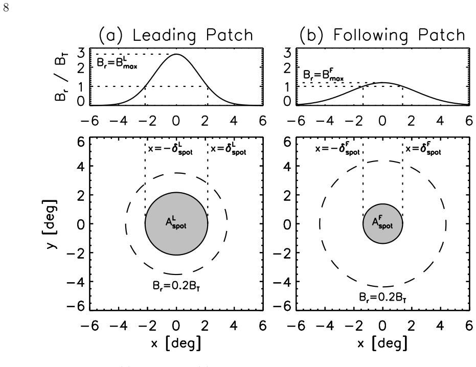
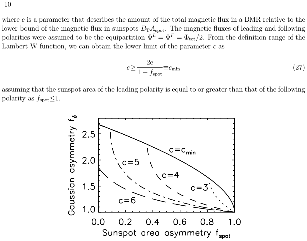
The central object is the bipolar magnetic region (BMR) modeled as two Gaussian magnetic patches of widths $\delta_L$ and $\delta_F$ with flux balance $B_{\max}^L(\delta_L)^2 \sim B_{\max}^F(\delta_F)^2$, so the following patch is wider and weaker when its sunspot area is smaller. The asymmetry parameter is $f_\delta = (\delta_F/\delta_L)^2$, tied to the observed sunspot area ratio $f_{\rm spot}$ through a Lambert-W inversion that yields the Gaussian width and peak field from area and flux. The diagnostic that carries the argument is the southern net hemispheric flux after five years: it measures how much cross-equatorial magnetic flux a BMR delivers to the polar field. The paper also uses the one-dimensional azimuthally averaged surface flux transport equation, whose linearity lets the authors calibrate the initial condition and threshold field by least squares and grid-search the remaining parameters.

What would settle it

Run the same surface flux transport hindcasts for cycles 21–24 using a following-to-leading sunspot area ratio of 0.8 (the alternative observational estimate) or with a flux-area scaling parameter above its minimum; if the axial dipole error no longer improves by 30–40 percent relative to the symmetric model, the central claim is refuted. A direct test would measure the magnetic-flux-weighted width ratio of leading versus following polarity patches in synoptic magnetograms and compare it with the model's inferred $f_\delta$.

Watch

Extended reading notes

Core claim

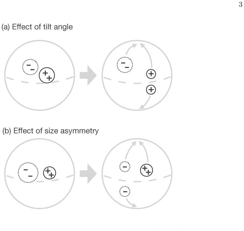
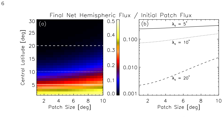
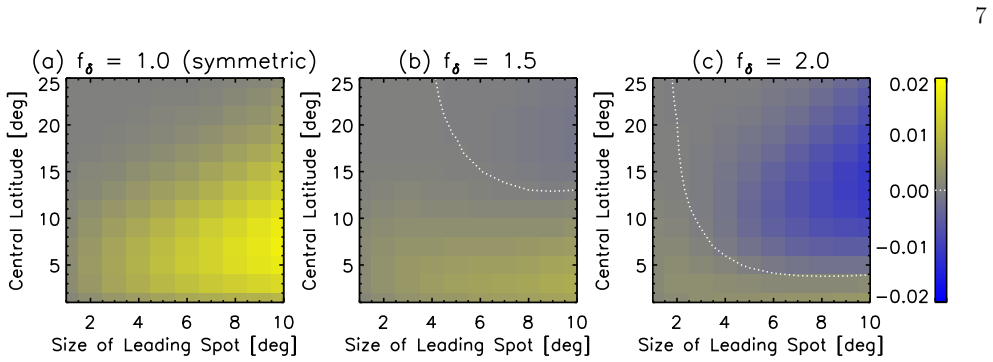
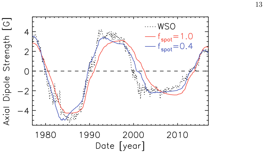
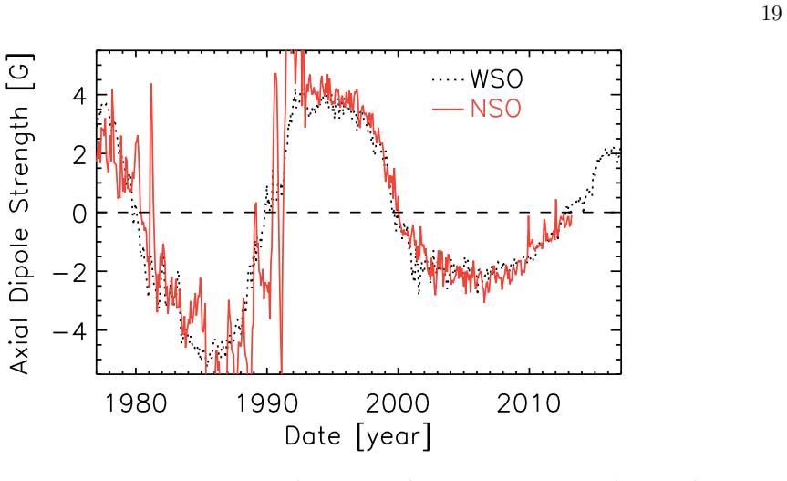
The central claim is that the morphological asymmetry between leading and following sunspots has a significant, previously neglected effect on the evolution of the large-scale surface magnetic field. Because magnetic flux is balanced between the two polarities, a smaller following sunspot area implies a wider, more diffuse following magnetic patch; that wider patch is disproportionately carried across the equator by diffusion and meridional flow, canceling the leading-polarity flux that normally builds the polar field. For large, high-latitude bipolar regions the effect is strong enough that strongly asymmetric BMRs reverse the regular polar field formation. In simulations driven by the observed sunspot record for cycles 21–24, the asymmetric model reduces the RMS difference of the axial dipole strength from WSO observations by 30–40 percent compared with the symmetric model, and shifts the timing of polar field reversal closer to observations.

Load-bearing premise

The reported 30–40 percent improvement rests on assuming the true sunspot area asymmetry is about 0.4 (following spot 40 percent as large as leading spot) and on a particular conversion from spot area to magnetic patch width whose free parameter the optimization pins to its lower bound; if the real asymmetry is milder, as one competing study suggests, the improvement could shrink or vanish.

Editorial extensions

If this is right

Standard surface flux transport models that assume symmetric spots overestimate polar field buildup and underestimate how much following-polarity flux reaches the poles, especially in cycles with large, high-latitude BMRs.
The timing of polar field reversal shifts: with asymmetry, the axial dipole begins to decline before the end of the cycle rather than amplifying to the end, matching observed profiles.
Solar cycle predictions based on polar field precursors should include spot size asymmetry, otherwise the predicted amplitude of the next cycle can be systematically off.
The long flat minimum between cycles 23 and 24 can be reproduced by the asymmetric model, suggesting asymmetry as a candidate explanation for weak, prolonged minima.
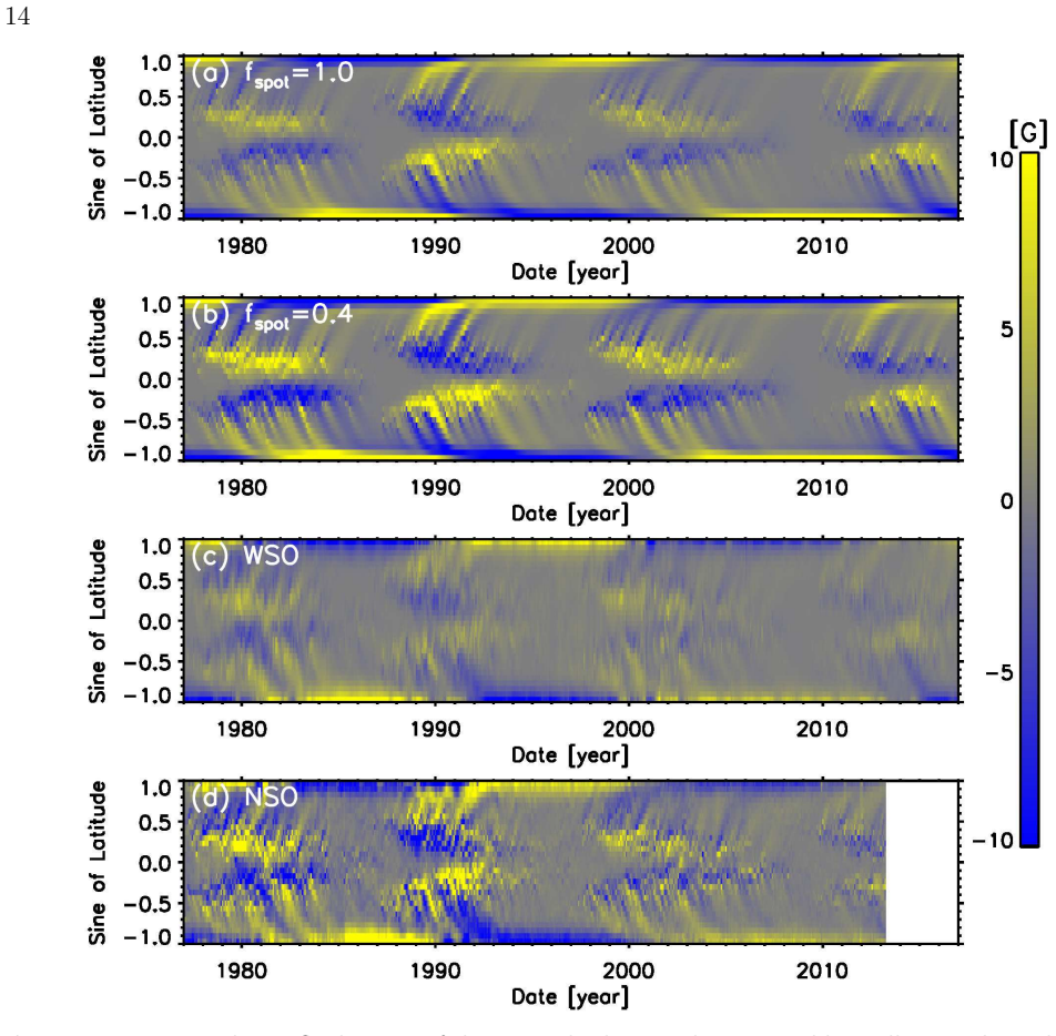
The asymmetry increases the grainy structure in the activity belts of the butterfly diagram, offering a partial explanation for observed low-latitude flux concentrations without raising high-latitude net flux.

Reading between the lines

Editorial extensions of the paper, not claims the author makes directly.

If this effect is as large as reported, the magnetic-flux-weighted width of following-polarity patches in synoptic magnetograms should systematically exceed that of leading patches; this is directly testable without relying on sunspot area catalogs.
The 30–40 percent improvement may partially absorb other missing physics, such as tilt-angle scatter or active region inflow; a model that includes both effects together could attribute the gain more precisely.
Because the asymmetry decays on a timescale of roughly a month for typical spots, and more slowly for large BMRs, cycle-to-cycle variation in the population of large active regions could drive part of the observed variability in polar field timing, independent of tilt angle.
A natural next test is to build cycle 25 hindcasts with the asymmetric source term and compare the predicted polar field and next-cycle amplitude against observations, using the inferred asymmetry as a free parameter per hemisphere.

Share X Bluesky LinkedIn Reddit HN

Signed reviews

No signed human review yet.

Editorial analysis

A structured set of objections, weighed in public.

Desk editor's note, referee report, and a circularity audit.

Desk Editor's Note

read the letter

The asymmetry effect is real and previously underappreciated, but the 30–40% improvement is an in-sample fit, not a predictive result. The single-BMR experiments in Section 3 are the core of the paper and they're solid. A wider following spot dumps more flux across the equator, and for large, high-latitude BMRs it can reverse the polar-field contribution. That is a genuine new result, and the paper is the first to quantify it in an SFT context. The derivation in Section 4 connecting area asymmetry fspot to patch-size asymmetry fδ via the Lambert W function is neat, and Appendix B gives a simple diffusion argument for why larger BMRs keep the asymmetry longer.

The soft spot is the quantitative claim in Section 5. The 30–40% RMS reduction is computed after a grid search over BT, c, and T21–T24 that minimizes the L2 difference to the WSO axial dipole on the same data used for the error. That is in-sample fitting, not a predictive test. Both optimized cases sit at the lower boundary of c, and the cycle-dependent tilts shift, so the improvement could be purchased by parameter changes rather than by the asymmetry physics isolated in Section 3. No cross-validation, bootstrap, or sensitivity analysis is provided, and the paper itself concedes the asymmetric model deviates from the observed polar field near the end of Cycle 21. The fspot choice is also a single value (0.4 from Tlatov et al.); using Muraközy et al.'s 0.8 would weaken the effect, as the paper notes.

That said, the limitations section is honest, the data calibration is careful, and the citation pattern is appropriate. This is a paper that a serious referee should engage with, but the verdict should be conditional: the mechanism is plausible, the quantitative improvement is not yet established. For a revision, I'd ask for an out-of-sample test (e.g., fit on cycles 21–23, score on 24) and a sensitivity scan over fspot and c. The paper is worth bringing to a reading group and citing for the effect, but not as evidence for a 30–40% prediction gain.

Recommendation: send to peer review, but insist on the sensitivity analysis before publishing the headline number.

Referee Report

3 major / 4 minor

Summary. The paper investigates whether the well-known morphological asymmetry between leading and following sunspots affects polar-field formation and solar-cycle prediction. Using a one-dimensional surface flux transport model, the authors first isolate the effect of a single bipolar magnetic region (BMR) and show that a larger, more diffuse following polarity reduces or even reverses the net cross-equatorial flux that builds the polar field, especially for large and high-latitude BMRs (Section 3). They then convert an observed sunspot-area asymmetry fspot into the model's patch-size asymmetry fdelta via a flux-area scaling with a parameter c (Section 4), and run simulations for Cycles 21-24, optimizing free parameters against the Wilcox Solar Observatory axial dipole series (Section 5). The paper reports a 30--40 percent reduction in RMS axial-dipole error when the asymmetry is included, while also acknowledging uncertainties in fspot and a remaining discrepancy in the polar field near the end of Cycle 21 (Section 6).

Significance. If the quantitative claim were established, the paper would be important: standard SFT models treat leading and following polarities as symmetric, and the paper's Section 3 experiments show a clean, parameter-free mechanism by which size asymmetry changes cross-equatorial flux and the timing of polar-field reversal. This mechanism is genuinely new in the SFT context and is supported by the isolated single-BMR simulations. The manuscript also makes a falsifiable qualitative prediction that asymmetric BMRs contribute less to the polar field, which deserves credit. However, the headline 30--40 percent RMS improvement is not yet established as a property of the asymmetry itself: it comes from an in-sample optimization of several free parameters against the same axial dipole series used to compute the error, and the solution sits on the boundary of the allowed parameter range. The qualitative conclusion is sound; the quantitative conclusion needs additional validation.

major comments (3)

[§5, Table 2 and Fig. 7] The 30--40 percent improvement reported in the Abstract and Section 5 is an in-sample fit residual, not a predictive test. The same WSO axial dipole time series is used both to optimize BT, c-cmin, and the cycle-dependent tilt factors T21-T24 and to compute the RMS error; no cross-validation, holdout, bootstrap, or sensitivity analysis is presented. Because the asymmetric case also has different optimized parameters and sits at c-cmin = 0, the reduction from 3.50 G to 2.18 G cannot be uniquely attributed to the asymmetry mechanism rather than to the parameter freedom absorbed by the fit. The authors should provide an out-of-sample or cross-validated assessment, or at least a parameter-sensitivity analysis showing that the improvement is stable when the fitted parameters are perturbed.
[§4.2, Eq. (27), and Table 2] The total-flux factor c is optimized to the lower boundary cmin in both the symmetric and asymmetric cases in Table 2, meaning the reported improvement relies on the flux-area relation Phi_tot = c BT Aspot at exactly the boundary of the Lambert-W existence range. This is a delicate point: the boundary value cmin = 2e/(1+fspot) forces the peak field Bmax to take a specific value, and the asymmetric case therefore uses a different total flux per spot area than the symmetric case. The paper does not justify why the physical system should sit at this boundary, nor does it explore the sensitivity of the 30--40 percent improvement to the assumed flux-area scaling. Showing results for c above cmin, or for an independently calibrated relation between spot area and flux, would substantially strengthen the quantitative claim.
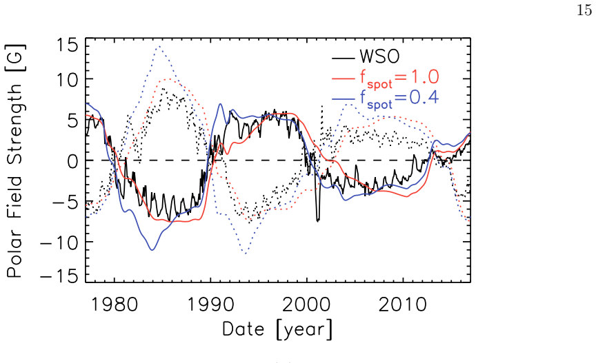
[§6] The quantitative conclusion is heavily contingent on the adopted value fspot = 0.4, which is not optimized but fixed using Tlatov et al. (2014). The paper itself notes that Muraközy et al. (2014) implies fspot ~ 0.8, which would produce a much weaker asymmetry, and that the asymmetric simulation deviates from the observed polar field near the end of Cycle 21. These concessions mean that the reported 30--40 percent error reduction may shrink or disappear under a reasonable alternative observational input. The authors should either quantify how the RMS error changes with fspot (e.g., a sweep over fspot = 0.4, 0.6, 0.8, 1.0) or substantially soften the abstract's numerical claim.

minor comments (4)

[Title] The title uses 'sun spots' as two words, while the abstract and body use 'sunspot'; the spelling should be made consistent.
[§3.2, Fig. 3 caption] The sentence 'In the weakly asymmetric case (fdelta = 1.5; Fig. 3b), the amount of the cross-equatorial flux becomes smaller than the asymmetric case' should read 'smaller than in the symmetric case', since the comparison is with fdelta = 1.0.
[§6] The text 'We used delta_spot = 0.4 as the typical ratio between the leading and following sunspot areas' appears to refer to fspot, the area ratio, not delta_spot, and should be corrected.
[§4.2, Eq. (26)] The definition Phi_tot = c BT Aspot is a strong modeling assumption; the paper would benefit from a brief discussion of how this form relates to previous SFT parameterizations and what range of c is physically plausible from sunspot magnetic-field observations.

Circularity Check

1 steps flagged · score 6.0 of 10

The 30–40% improvement is an in-sample fit residual: Table 2 parameters are optimized against the same WSO axial dipole series used to compute the RMS error.

fitted input called prediction [Abstract; §5 'Effect of Asymmetry in Whole Solar Cycle', Table 2 and Fig. 7]
"Using the linearity of the SFT model on the magnetic field, we determined the strength of the initial condition and threshold strength of the magnetic field BT by minimizing the L2-norm of the difference between the simulated and observed axial dipole strengths. The WSO synoptic magnetogram was used as the reference observation. We optimized other free parameters using the grid search with the parameter range and step size given in Table 1. The optimal parameters and residual errors are shown in Table 2."

The reported 30–40% reduction is not a predictive test: the same WSO axial dipole series is both the optimization target for {BT, c, T21–T24} and the data used to compute the RMS errors in Table 2. The fspot=0.4 and fspot=1.0 cases are compared by their in-sample residuals after grid searches on that same target, so a lower residual for the asymmetric model is a fit result that can be purchased by parameter shifts, not an out-of-sample property of the asymmetry. The non-circular §3 experiments establish the mechanism, but they do not validate the 30–40% number. In addition, the asymmetric optimum sits at the boundary c−cmin=0 (Table 2), maximizing fδ for fixed fspot, and the cycle tilt factors also differ, so the improvement is not isolated to the morphology physics.

full rationale

The mechanistic Section 3 is self-contained: the single-BMR experiments (Fig. 3) show from the model equations that making the following Gaussian patch wider reduces or reverses the cross-equatorial flux contribution, and this does not depend on any fit to the WSO series. That part is not circular and provides independent content. The 30–40% improvement in the abstract and §5, however, is a comparison of two optimization residuals: the same WSO axial dipole series is used both as the target for minimizing the L2 norm (for BT, c, and cycle-dependent tilts T21–T24) and as the yardstick for the reported RMS errors in Table 2. No out-of-sample or cross-validated prediction is made, and Fig. 7 simply overlays the optimized hindcasts on the fitting data. The asymmetric optimum also lands at the boundary c−cmin=0 (Table 2), maximizing the model's fδ for the adopted fspot=0.4, so the error reduction is not isolated from the extra freedom in parameter space. The paper itself concedes in §6 that 'as we optimized the solutions by minimizing the difference from the observed axial dipole strength, it was not guaranteed that the optimized solution would also demonstrate good correspondence with the observed polar magnetic field strength.' Thus the central mechanistic insight is supported independently, but the headline quantitative reduction is a fitted-input-called-prediction step, giving a partial circularity score of 6 rather than a fully circular result.

Assumptions & free parameters 5 free parameters · 5 assumptions · 0 invented entities

The central claim rests on several modeling assumptions, most notably the Gaussian BMR profile, the flux-area scaling with a free parameter c, and the fixed area asymmetry fspot=0.4. The model also has five fitted parameters (BT, c, T21-T24, initial condition strength). No new physical entities are invented. The flux-area scaling is the most ad hoc element, as it is introduced to bridge observations and model parameters without direct validation.

free parameters (5)

fspot (sunspot area asymmetry) = 0.4
Set to the typical observed value from Tlatov et al. 2014, not optimized in this paper. The quantitative improvement depends on this value; a value of 0.8 from Muraközy et al. 2014 would weaken the effect.
BT (threshold magnetic field strength) = 1670 G (asymmetric case), 1830 G (symmetric case)
Optimized via L2 minimization against WSO axial dipole in Section 5.
c (total flux factor) = c - cmin = 0.0 (c = 2e/(1+fspot), about 3.88 for fspot=0.4)
Optimized via grid search; hit the lower bound in both cases, indicating the best fit lies at the edge of the allowed range.
T21-T24 (cycle-dependent tilt factors) = 1.4, 1.5, 1.3, 1.6 (asymmetric case)
Optimized via grid search to capture cycle-to-cycle differences in mean tilt angle.
Initial condition strength = Not reported explicitly
Determined by minimizing the L2 difference to the observed axial dipole; a free scaling parameter of the quasi-steady initial condition.

assumptions (5)

domain assumption The SFT equation (Eq. 1) with the given meridional flow and diffusion coefficient (250 km2/s) captures the relevant surface magnetic field evolution.
Standard model used throughout solar physics; the paper relies on it to translate BMR asymmetries into polar field changes.
domain assumption A BMR is adequately represented as two Gaussian magnetic patches with a specific profile (Eq. 3) and the parameters of each patch are determined by flux balance (Eq. 11).
This profile is a modeling assumption; real sunspot fields are not exactly Gaussian. The paper acknowledges this in Section 6.
ad hoc to paper The sunspot area asymmetry fspot can be converted to patch size asymmetry fdelta using the flux-area relation Phi_tot = c BT Aspot (Eq. 26) and equal flux partition between polarities.
This relation is introduced to connect observed areas to the model's Gaussian widths; it introduces the parameter c that must be fitted. The paper does not validate this scaling against direct observations.
domain assumption The tilt angle law alpha = g_inflow Tn sqrt(|lambda|) (with g_inflow=0.7 and cycle-dependent Tn) is an adequate representation of Joy's law with active region inflow.
Taken from Cameron et al. 2010; the paper fits Tn per cycle.
standard math The one-dimensional azimuthally averaged SFT model exactly reproduces the evolution of the azimuthally averaged field for axisymmetric velocity and diffusion.
Based on Cameron & Schüssler 2007; the paper uses this to justify the 1D model.

how reviews work

0 comments

Cite this review

Pith. "Pith review of Effect of morphological asymmetry between leading and following sunspots on the prediction of solar cycle activity." pith.science (2026). https://pith.science/paper/3XL2W7CB

@misc{pith2026190804474,
  author       = {Pith},
  title        = {Pith review of: Effect of morphological asymmetry between leading and following sunspots on the prediction of solar cycle activity},
  year         = {2026},
  howpublished = {\url{https://pith.science/paper/3XL2W7CB}},
  note         = {Machine review of arXiv:1908.04474}
}

read the original abstract

The morphological asymmetry of leading and following sunspots is a well-known characteristic of the solar surface. In the context of large-scale evolution of the surface magnetic field, the asymmetry has been assumed to have only a negligible effect. Using the surface flux transport model, we show that the morphological asymmetry of leading and following sunspots has a significant impact on the evolution of the large-scale magnetic field on the solar surface. By evaluating the effect of the morphological asymmetry of each bipolar magnetic region (BMR), we observe that the introduction of the asymmetry in the BMR model significantly reduces its contribution to the polar magnetic field, especially for large and high-latitude BMRs. Strongly asymmetric BMRs can even reverse the regular polar field formation. The surface flux transport simulations based on the observed sunspot record shows that the introduction of the morphological asymmetry reduces the root-mean-square difference from the observed axial dipole strength by 30--40 percent. These results indicate that the morphological asymmetry of leading and following sunspots has a significant effect on the solar cycle prediction.

Figures

Figures reproduced from arXiv: 1908.04474 by the authors.

**Figure 1.** Schematic illustration of the effects of the sunspot tilt angle (panel a) and size asymmetry (panel b) on the cross-equatorial flux transport and formation of the polar magnetic field. Thin gray arrows indicate the poleward transport by the meridional flow. 2.1. Basic equation The basic equation of the one-dimensional version of the SFT model can be written as ∂BR ∂t + 1 R⊙ sin θ ∂ ∂θ (BRVθ sin θ) = 1 R2 ⊙ sin θ ∂ ∂… view at source ↗

**Figure 2.** Contribution of a Gaussian magnetic patch to the polar magnetic field (southern net hemispheric flux after five years that is normalized by the magnetic flux of initial patch). Panel a: normalized hemispheric flux as a function of the size δ and central latitude λc of the magnetic patch at the initial state. Horizontal white lines show the central latitude of 5 (solid), 10 (dotted), and 20 (dashed) [deg]. Panel b: n… view at source ↗

**Figure 3.** Effect of the asymmetric sunspots on the contribution to the polar magnetic field by the emergence of a single BMR. Illustrated are the net hemispheric fluxes after five years normalization by the total (leading + following) unsigned magnetic flux of the BMR with (a) fδ = 1.0 (symmetric case), (b) fδ = 1.5 (weakly asymmetric case), and (c) fδ = 2.0 (strongly asymmetric case). The white dotted lines indicate the loca… view at source ↗

Figures from the paper (8 more)

**Figure 4.** Figure 4: Example of (a) leading and (b) following magnetic patch in the BMR model used in Sections 4 and 5. Top panels show the cross sections of the magnetic patches across each peak position. Bottom panels show the two-dimensional profile of the modeled magnetic patch. The re…

**Figure 5.** Figure 5: Relation between the asymmetries of patch sizes in the BMR model and observed sunspot area. Each line represents a different value of c = Φtot/(BTAspot). Depicted are the cases with c = cmin = 2e/(1 + fspot) (solid), c = 3 (dotted), c = 4 (dashed), c = 5 (dash-dotted),…

**Figure 6.** Figure 6: Dependence of (a) the normalized average magnetic field strength in sunspots BT/BT and (b) the ratio between the total magnetic flux and sunspot flux Φtot/(BspotAspot) on the total flux factor c = Φtot/(BTAtot). Depicted are fspot = 2e/c − 1 (solid), fspot = 10−3 (dott…

**Figure 7.** Figure 7: Axial dipole strength of the optimal solutions shown in [PITH_FULL_IMAGE:figures/full_fig_p013_7.png]

**Figure 8.** Figure 8: Magnetic butterfly diagram of the optimal solutions shown in [PITH_FULL_IMAGE:figures/full_fig_p014_8.png]

**Figure 9.** Figure 9: Polar magnetic field strength averaged over |λ|≥55 of the optimal solutions shown in [PITH_FULL_IMAGE:figures/full_fig_p015_9.png]

**Figure 10.** Figure 10: Axial dipole strength of the WSO (black dotted) and calibrated NSO (red solid) synoptic magnetograms [PITH_FULL_IMAGE:figures/full_fig_p019_10.png]

**Figure 11.** Figure 11: Polar magnetic field strength averaged over |λ|≥55 of the WSO (black) and calibrated NSO (red) synoptic maps. The polar fields in the northern and southern hemispheres are shown by solid and dashed lines, respectively. REFERENCES Babcock, H. W. 1961, ApJ, 133, 572 Bau…

Discussion (0). Continue with ORCID to comment.

Forward citations

Cited by 1 Pith paper

Reviewed papers in the Pith corpus that reference this work. Sorted by Pith novelty score. Full citation record

Constraining the radial decay timescale of solar surface magnetic field through a comparative study of data-assimilative 2D surface flux transport and 3D dynamo models
astro-ph.SR 2026-07 conditional novelty 6.0 of 10

A comparative analysis of 2D surface flux transport and 3D dynamo models yields a mode-dependent radial decay spectrum with effective timescales τ≈2 yr (l=8) for magnetogram assimilation and τ≈7 yr (dipole) for active...

Reference graph

Works this paper leans on

50 extracted references · 47 canonical work pages · cited by 1 Pith paper

[1]

Babcock, H. W. 1961, ApJ, 133, 572

1961
[2]

2006, A&A, 446, 307

Baumann, I., Schmitt, D., & Sch¨ ussler, M. 2006, A&A, 446, 307

work page 2006
[3]

Solanki, S. K. 2004, A&A, 426, 1075

work page 2004
[4]

1995, ApJ, 441, 886 20

Caligari, P., Moreno-Insertis, F., & Schussler, M. 1995, ApJ, 441, 886 20

work page 1995
[5]

2007, ApJ, 659, 801

Cameron, R., & Sch¨ ussler, M. 2007, ApJ, 659, 801

work page 2007
[6]

H., Dasi-Espuig, M., Jiang, J., et al

Cameron, R. H., Dasi-Espuig, M., Jiang, J., et al. 2013, A&A, 557, A141

work page 2013
[7]

H., Jiang, J., Schmitt, D., & Sch¨ ussler, M

Cameron, R. H., Jiang, J., Schmitt, D., & Sch¨ ussler, M. 2010, ApJ, 719, 264

work page 2010
[8]

H., Jiang, J., & Sch¨ ussler, M

Cameron, R. H., Jiang, J., & Sch¨ ussler, M. 2016, ApJL, 823, L22

work page 2016

Show all 50 references

[9]

1998, in Astronomical Society of the Paciﬁc Conference

Cauzzi, G., & van Driel-Gesztelyi, L. 1998, in Astronomical Society of the Paciﬁc Conference

1998
[10]

2017, ApJ, 846, 149

Chen, F., Rempel, M., & Fan, Y. 2017, ApJ, 846, 149

2017
[11]

2008, ApJ, 676, 680 —

Fan, Y. 2008, ApJ, 676, 680 —. 2009, Living Reviews in Solar Physics, 6, 4

2008
[12]

H., & Deluca, E

Fan, Y., Fisher, G. H., & Deluca, E. E. 1993, ApJ, 405, 390

1993
[13]

H., Fan, Y., Longcope, D

Fisher, G. H., Fan, Y., Longcope, D. W., Linton, M. G., & Pevtsov, A. A. 2000, SoPh, 192, 119

2000
[14]

2018, Journal of Atmospheric and Solar-Terrestrial Physics, 176, 26

Akiyama, S. 2018, Journal of Atmospheric and Solar-Terrestrial Physics, 176, 26

2018
[15]

I., & Shu, C.-W

Gottlieb, S., Ketcheson, D. I., & Shu, C.-W. 2009, Journal of Scientiﬁc Computing, 38, 251

2009
[16]

1950, ZA, 28, 28

Grotrian, W., & K¨ unzel, H. 1950, ZA, 28, 28

1950
[17]

A., Hindman, B

Haber, D. A., Hindman, B. W., Toomre, J., et al. 2002, ApJ, 570, 855

2002
[18]

E., Ellerman, F., Nicholson, S

Hale, G. E., Ellerman, F., Nicholson, S. B., & Joy, A. H. 1919, ApJ, 49, 153

1919
[19]

Hathaway, D. H. 2015, Living Reviews in Solar Physics, 12, 4

2015
[20]

H., & Rightmire, L

Hathaway, D. H., & Rightmire, L. 2011, ApJ, 729, 80

2011
[21]

H., & Upton, L

Hathaway, D. H., & Upton, L. A. 2016, Journal of Geophysical Research (Space Physics), 121, 10

2016
[22]

H., Wilson, R

Hathaway, D. H., Wilson, R. M., & Reichmann, E. J. 1999, J. Geophys. Res., 104, 22

1999
[23]

2018, ApJL, 864, L5

Imada, S., & Fujiyama, M. 2018, ApJL, 864, L5

2018
[24]

H., Schmitt, D., & Sch¨ ussler, M

Jiang, J., Cameron, R. H., Schmitt, D., & Sch¨ ussler, M. 2011, A&A, 528, A82 —. 2013, SSRv, 176, 289

2011
[25]

H., & Sch¨ ussler, M

Jiang, J., Cameron, R. H., & Sch¨ ussler, M. 2014a, ApJ, 791, 5 —. 2015, ApJL, 808, L28

2015
[26]

2018, ApJ, 863, 159 Mu˜ noz-Jaramillo, A., Balmaceda, L

Jiang, J., Wang, J.-X., Jiao, Q.-R., & Cao, J.-B. 2018, ApJ, 863, 159 Mu˜ noz-Jaramillo, A., Balmaceda, L. A., &

2018
[27]

DeLuca, E. E. 2013, Physical Review Letters, 111, 041106 Mu˜ noz-Jaramillo, A., Sheeley, N. R., Zhang, J., &

2013
[28]

DeLuca, E. E. 2012, ApJ, 753, 146 Mu˜ noz-Jaramillo, A., Senkpeil, R. R.,

2012
[29]

C., et al

Windmueller, J. C., et al. 2015, ApJ, 800, 48 Murak¨ ozy, J., Baranyi, T., & Ludm´ any, A. 2014, SoPh, 289, 563

2015
[30]

Pesnell, W. D. 2012, SoPh, 281, 507

2012
[31]

Petrie, G. J. D. 2015, Living Reviews in Solar Physics, 12, 5

2015
[32]

2010, Living Reviews in Solar Physics, 7, 6

Petrovay, K. 2010, Living Reviews in Solar Physics, 7, 6

2010
[33]

Rempel, M., & Cheung, M. C. M. 2014, ApJ, 785, 90

2014
[34]

2005, Geophys

Schatten, K. 2005, Geophys. Res. Lett., 32, L21106

2005
[35]

Wilcox, J. M. 1978, Geophys. Res. Lett., 5, 411

1978
[36]

J., De Rosa, M

Schrijver, C. J., De Rosa, M. L., & Title, A. M. 2002, ApJ, 577, 1006

2002
[37]

J., & Liu, Y

Schrijver, C. J., & Liu, Y. 2008, SoPh, 252, 19

2008
[38]

W., & Kamide, Y

Svalgaard, L., Cliver, E. W., & Kamide, Y. 2005, Geophys. Res. Lett., 32, L01104

2005
[39]

A., & Mursula, K

Pevtsov, A. A., & Mursula, K. 2015, Advances in Space Research, 55, 835

2015
[40]

G., Vasil’eva, V

Tlatov, A. G., Vasil’eva, V. V., Makarova, V. V., & Otkidychev, P. A. 2014, SoPh, 289, 1403

2014
[41]

Priest, E. R. 1998, ApJ, 501, 866 van Driel-Gesztelyi, L., & Petrovay, K. 1990, SoPh, 126, 285

1998
[42]

2017, A&A, 604, A8

Yeates, A., & Mursula, K. 2017, A&A, 604, A8

2017
[43]

Wang, Y.-M., Robbrecht, E., & Sheeley, Jr., N. R. 2009, ApJ, 707, 1372

2009
[44]

Wang, Y.-M., & Sheeley, N. R. 2009, ApJL, 694, L11

2009
[45]

A., Fan, Y., & Miesch, M

Weber, M. A., Fan, Y., & Miesch, M. S. 2011, ApJ, 741, 11

2011
[46]

R., Mu˜ noz-Jaramillo, A., & Petrie, G

Whitbread, T., Yeates, A. R., Mu˜ noz-Jaramillo, A., & Petrie, G. J. D. 2017, A&A, 607, A76 21

2017
[47]

R., Baker, D., & van Driel-Gesztelyi, L

Yeates, A. R., Baker, D., & van Driel-Gesztelyi, L. 2015, SoPh, 290, 3189

2015
[48]

S., Fainshtein, V

Zagainova, Y. S., Fainshtein, V. G., Obridko, V. N., & Rudenko, V. G. 2017, Geomagnetism and Aeronomy, 57, 946

2017
[49]

Zhao, J., & Kosovichev, A. G. 2004, ApJ, 603, 776

2004
[50]

1981, NASA Special Publication, 450

Zwaan, C. 1981, NASA Special Publication, 450

1981

Pith tools

Reviewed August 14, 2026 · model on record in the stance chip above.

[1] [1]

Babcock, H. W. 1961, ApJ, 133, 572

1961

[2] [2]

2006, A&A, 446, 307

Baumann, I., Schmitt, D., & Sch¨ ussler, M. 2006, A&A, 446, 307

work page 2006

[3] [3]

Solanki, S. K. 2004, A&A, 426, 1075

work page 2004

[4] [4]

1995, ApJ, 441, 886 20

Caligari, P., Moreno-Insertis, F., & Schussler, M. 1995, ApJ, 441, 886 20

work page 1995

[5] [5]

2007, ApJ, 659, 801

Cameron, R., & Sch¨ ussler, M. 2007, ApJ, 659, 801

work page 2007

[6] [6]

H., Dasi-Espuig, M., Jiang, J., et al

Cameron, R. H., Dasi-Espuig, M., Jiang, J., et al. 2013, A&A, 557, A141

work page 2013

[7] [7]

H., Jiang, J., Schmitt, D., & Sch¨ ussler, M

Cameron, R. H., Jiang, J., Schmitt, D., & Sch¨ ussler, M. 2010, ApJ, 719, 264

work page 2010

[8] [8]

H., Jiang, J., & Sch¨ ussler, M

Cameron, R. H., Jiang, J., & Sch¨ ussler, M. 2016, ApJL, 823, L22

work page 2016