REVIEW 3 major objections 6 minor 62 references
Invasion Fronts Outside the Homoclinic Snaking Region in the Planar Swift-Hohenberg Equation
T0 review · 3 major / 6 minor · reviewed 2026-08-14 · deepseek-v4-flash
Pith's one-line read Invading stripe fronts in the Swift-Hohenberg equation select a unique speed and wavenumber, while retreating fronts form one-parameter families.
desk verdict A serious, publishable numerical study of depinning fronts with genuinely new results; the numerics are careful and the theory is honestly conditional on an unverified transversality assumption. read the letter →
The pith
A machine-rendered reading of the paper's core claim, the machinery that carries it, and where it could break.
The reading
What carries the argument
The load-bearing object is the far-field core decomposition, which writes a front as the product of a far-field stripe $u_s(k_x(\rho\pm\tau+\psi);k_x)$ with a cut-off $\chi(\rho)$ plus a remainder $v(\rho,\tau;\omega)$ that is localised near the interface. Posed in exponentially weighted spaces $L^2_\alpha$, this makes the linearised operator Fredholm so that Newton and continuation methods apply, with two integral phase conditions fixing the translational mode and the far-field wavenumber; the unknowns solved for are the remainder $v$, the wavenumber $k_x$, and the transition frequency $\omega=c k_x$. The proof of Proposition 1.1 uses a Lyapunov-Schmidt reduction in this setup, and the stationary selection theory enters through the conserved quantities $H(u)$ and $S(u)$ that force a stationary front's far-field stripes to sit on the zero-Hamiltonian set.
What would settle it
Compute, at a numerically converged invasion front for representative parameters in the bistable region, the eigenvalues and eigenfunctions of the linearised operator $L$ in the exponentially weighted space $L^2_{-\alpha}$; an extra near-zero eigenvalue, or a zero eigenvalue of algebraic multiplicity greater than one, would refute Hypothesis 3 and with it the uniqueness part of Proposition 1.1. A second, independent test is to run two time simulations starting from fronts with different initial stripe wavenumbers or phases and check whether both converge to the same $c$ and $k_x$.
Extended reading notes
Core claim
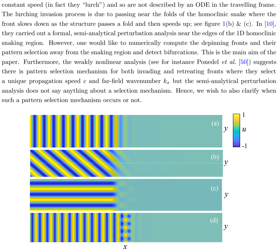
The paper's main result is a pattern-selection dichotomy for parallel depinning fronts. Assuming the far-field stripe is temporally stable and the front is transverse, an invading front survives small perturbations and selects a unique invasion speed $c$ and far-field wavenumber $k_x$ for fixed $\mu$ and $\nu$; a retreating front instead forms a one-parameter family parameterised by $k_x$, with $c=c(k_x)$. The numerical companion result, obtained by solving the far-field core decomposition boundary-value problem, is that almost-planar invasion fronts in the cubic-quintic Swift-Hohenberg equation (nonlinearity $f(u)=\nu u^3-u^5$) bifurcate from parallel invasion fronts and coexist close to the homoclinic snaking region, while far away no almost-planar fronts exist and parallel fronts can regain transverse stability once they propagate above a critical speed.
Load-bearing premise
The result assumes a transversality condition (Hypothesis 3): the kernel of the linearisation about the front in $L^2_{-\alpha}$ is exactly two-dimensional, spanned by spatial and temporal translations, and the zero eigenvalue is algebraically simple; the paper states this without proving it for the Swift-Hohenberg equation.
Editorial extensions
If this is right
- Invading parallel depinning fronts can be path-followed in $(c,k_x,\mu,\nu)$-space, so folds and stability changes are located by continuation rather than inferred from time simulations.
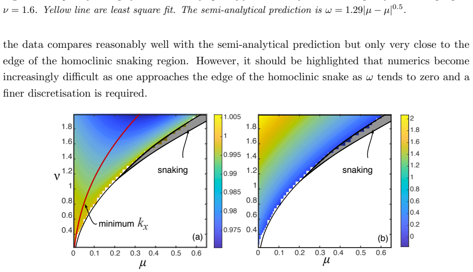
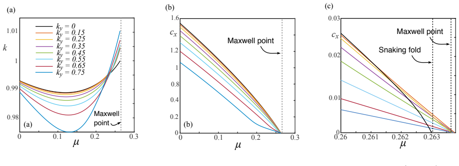
- The selected wavenumber begins at the Hamiltonian-selected value at the snaking edge, dips, then increases; this non-monotonic dip is a quantitative target for exponential-asymptotic theories of pinning.
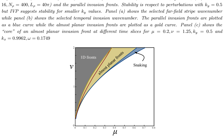
- Almost-planar invasion fronts exist only close to the snaking region, where they coexist with parallel fronts and travel slower; far away, parallel fronts are the only invasion mode and can become transversely stable at high speed.
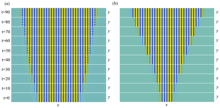
- Patch growth on the plane is governed by the parallel and perpendicular front speeds: the parallel front fixes the stepping rate in one direction while the perpendicular front sets the other, matching the observed bulging of growing stripe patches.
Reading between the lines
- If the pattern-selection dichotomy holds beyond the Swift-Hohenberg equation, then bistable pattern-forming systems generally have a computable invasion speed and wavelength, so patch morphology in reaction-diffusion or convection models could be predicted from front data alone.
- Hypothesis 3 could be certified numerically by solving the adjoint eigenvalue problem at the computed fronts; a numerical proof of a simple algebraically isolated zero eigenvalue would upgrade Proposition 1.1 from assumed to verified for the computed branches.
- The wavenumber dip near the snaking edge is consistent with exponentially small splitting between stable and unstable manifolds, suggesting that matched-asymptotics methods could predict the location and depth of the dip as a function of $\mu$ and $\nu$.
- The same boundary-value construction should apply to fronts whose far field is a different cellular pattern, such as hexagons, and to systems with nonlocal or discrete spatial structures, where the essential-spectrum obstruction is analogous.
Signed reviews
Editorial analysis
A structured set of objections, weighed in public.
Referee Report
Summary. The paper develops a numerical continuation framework for depinning (invasion) fronts in the planar Swift-Hohenberg equation in the bistable region outside homoclinic snaking. The main theoretical result is a conditional selection principle (Proposition 1.1): transversely invading parallel fronts are claimed to select a unique speed and far-field wavenumber, whereas retreating fronts are claimed to form one-parameter families. The numerical methodology adapts the far-field core decomposition of Lloyd & Scheel to moving fronts, adding phase conditions for the transition frequency and far-field wavenumber. Extensive computations are reported for parallel, oblique, perpendicular, and almost-planar fronts in the quadratic-cubic and cubic-quintic SH equations, including two-parameter sweeps, comparison to semi-analytical theory near the snaking edge, and application to the invasion of localized stripe patches.
Significance. If the claims are correct, the paper makes a valuable methodological contribution: it provides a concrete, systematic way to compute pattern-selecting invasion fronts in a class of pattern-forming PDEs, going beyond time-stepping and beyond the weakly nonlinear regime. The far-field core decomposition with phase conditions is a natural and useful extension of prior work, and the convergence studies for the 1D parallel-front solver (Figures 12-13) are careful and informative. The comparison with the semi-analytical |δ|^{1/2} scaling law (Figure 15) gives a meaningful benchmark, and the paper is honest about several open issues, including the lack of a proof of the needed transversality. However, the central uniqueness theorem rests on an unproved and, as stated, internally inconsistent transversality hypothesis, and the main numerical examples for the quadratic-cubic equation are computed in a regime that appears to violate the theorem's stability hypothesis. The almost-planar front coexistence, one of the headline observations, is supported only by computations at a single transverse resolution without a published convergence check.
major comments (3)
- [Appendix A.1, Hypothesis 3] Hypothesis 3 as stated is internally inconsistent: it says the kernel of L in L^2_{-α} is two-dimensional, spanned by ∂_ρ u* and ∂_τ u*, and then says the eigenvalue λ=0 is algebraically simple. A two-dimensional kernel in that space precludes algebraic simplicity of the zero eigenvalue. The proof of Proposition A.1 actually needs a different statement: in the exponentially weighted space L^2_α the kernel should be one-dimensional (e.g., spanned by an exponentially localized combination of ∂_ρ u* and ∂_τ u*) and the parameter derivatives (∂_{kx}, ∂_ψ, ∂_ω) F_v should cover the remaining cokernel directions of D F_v. The hypothesis as written is therefore not merely unverified but ill-posed, and it is load-bearing for the uniqueness part of Proposition 1.1. The convergence tests in Section 6.4 (Figures 12-13) certify discretization error of a single computed solution; they do not certify the absence of additional neutral modes. If an extra mode, such as a resonant stripe sideband, exists, the Lyapunov-Schmidt reduction of Proposition A.1 fails and the branches computed in Section 7 could be folds rather than genuine selection curves.
- [Proposition 1.1 and Section 7.1] The uniqueness/selection theorem assumes temporal stability of the far-field stripe solution, but the main numerical study of parallel fronts in Section 7.1 uses the quadratic-cubic SH equation at ν=1.6, for which the paper itself states (Section 2) that stripes are typically unstable in the bistable region to hexagonal perturbations. No argument is given to show that the hexagon instability is irrelevant for the 1D front problem, nor is the stability hypothesis verified for the computed branches. Consequently, the interpretation of Figure 14 as a confirmation of Proposition 1.1 is not supported by the stated hypotheses of that proposition. The paper needs to either restrict the theoretical claim to stable regimes, prove that the relevant stability notion is only the longitudinal one, or explicitly mark the quadratic-cubic results as being outside the theorem's assumptions.
- [Section 7.3, Figure 19] The claim that almost planar invasion fronts bifurcate off parallel fronts and coexist near the snaking region is a headline observation, but it is based on computations with N_γ = N_τ = 16 and no convergence study in the transverse direction. The parallel branch itself is reported to be zig-zag unstable for the whole bistable region (Figure 19, left panel), which makes it unclear whether the observed bifurcation is a genuine solution bifurcation or a numerical artifact from an under-resolved transverse discretization. The paper should provide a mesh-refinement study in γ and τ for the almost-planar branches, and it should report the extrapolated values of ω and k_x with error estimates at the reported fold location, before this claim can be considered quantitatively supported.
minor comments (6)
- [Lemma 1 and Proposition A.1] The text says 'invading fronts with ω<0' in Lemma 1 and in the statement of Proposition A.1, but throughout Section 6 and the introduction ω is defined as a positive quantity (ω = c k_x, c>0 for invading fronts). Please clarify the sign convention.
- [Section 1, paragraph after Figure 2] The manuscript says there are 'three types of possible depinning stripe fronts: parallel, oblique, perpendicular and almost-planar stripe fronts' but then lists four types; please correct the count or the list.
- [Section 6.4, equation (6.9)] The symbol L is used both for the linearized operator and for the domain length L_ρ; also the definition of L in (6.9) uses a minus sign before the biharmonic term while the operator in (6.7a) has a plus sign before it; please harmonize the notation.
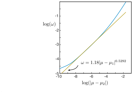
- [Figure 15] The fitted scaling law is reported as ω = 1.18 |μ-μ_1|^{0.5292} with no error bars or fit-quality measures; given that the exponent is expected to be 0.5, a confidence interval on the fitted exponent should be stated, along with the number of data points used and the residuals.
- [Section 7.3, last paragraph] The text states that 'IVP suggests stability for smaller ky values' but no supporting IVP results or stability computation is shown; please provide evidence or rephrase as a conjecture.
- [References] Several references are listed as 'Submitted 2018' or 'Submitted 2019'; if any have since appeared, please update them; otherwise state the status explicitly in the bibliography.
Circularity Check
No significant circularity: the selection theorem is explicitly conditional on a transversality hypothesis, and the numerics are self-contained rather than fitted to the claimed predictions.
full rationale
The paper's central claim, Proposition 1.1, is a conditional statement: it assumes temporal stability of the far-field stripes, existence of a transverse invasion front, and the explicit Hypothesis 3 in Appendix A.1 (kernel of the linearization spanned by the two translation modes, with the relevant zero eigenvalue algebraically simple). The Lyapunov-Schmidt reduction in Proposition A.1 is then a standard parameter-counting argument: L is Fredholm of index -1 for invading fronts (Lemma 1), the free parameters (kx, psi, omega) plus the two translation modes balance the cokernel, and the algebraic simplicity assumption is used to solve for omega. This is not circular because the hypothesis is a spectral nondegeneracy condition, not the selected values c and kx themselves. The numerical method of Section 6.4 solves for (v, omega, kx) as genuine unknowns with phase conditions; no fitted value is inserted as a predicted output. The least-squares fit in Figure 15 is a diagnostic comparison with the semi-analytic |delta|^{1/2} law, not a parameter used in the selection computation. The author's prior work [37] supplies the far-field core decomposition and continuation methodology, but that decomposition is a representation of any front (u = us chi + v) and the numerical results are new, with independent checks against weakly nonlinear travelling-front formulas from [26,50] and against initial-value simulations in Section 6.1. The unproved and potentially internally inconsistent statement of Hypothesis 3 is a genuine correctness/rigor risk for reading Proposition 1.1 as unconditional, but it is not circular reasoning: the paper states it as an assumption, not as a consequence of its derivation.
Assumptions & free parameters
free parameters (2)
- prefactor and exponent in the omega-scaling fit of Figure 15 =
1.18 and 0.5292
- domain truncation L_rho, cut-off d, grid sizes N_rho, N_tau, N_gamma =
L_rho=40 pi, d=20 to 40, N_rho=400, N_tau=20, N_gamma=16
assumptions (5)
- domain assumption Hypothesis 1: for an open region of kx the periodic stripe orbits are stable and the critical Floquet eigenvalue has expansion lambda = d_parallel eta^2 + O(eta^4).
- domain assumption Hypothesis 2: the trivial state is linearly stable, so mu > 0.
- domain assumption Hypothesis 3: for a front u*, the kernel of L in L^2_{-alpha} is two-dimensional, spanned by d_rho u* and d_tau u*, and the zero eigenvalue is algebraically simple.
- domain assumption Exponential convergence of the front to its asymptotic stripe and trivial states with a well-defined asymptotic phase.
- standard math Fredholm bordering and Lyapunov-Schmidt reduction for Fredholm index -1 problems.
Cite this review
Pith. "Pith review of Invasion Fronts Outside the Homoclinic Snaking Region in the Planar Swift-Hohenberg Equation." pith.science (2026). https://pith.science/paper/42AIDV7X
@misc{pith2026190808274,
  author       = {Pith},
  title        = {Pith review of: Invasion Fronts Outside the Homoclinic Snaking Region in the Planar Swift-Hohenberg Equation},
  year         = {2026},
  howpublished = {\url{https://pith.science/paper/42AIDV7X}},
  note         = {Machine review of arXiv:1908.08274}
}
read the original abstract
In this paper, we carry out numerical bifurcation analysis of depinning of fronts near the homoclinic snaking region, involving a spatial stripe cellular pattern embedded in a quiescent state, in the two-dimensional Swift-Hohenberg equation with either a quadratic-cubic or cubic-quintic nonlinearity. We focus on depinning fronts involving stripes that are orientated either parallel, oblique and perpendicular to the front interface, and almost planar depinning fronts. We show that invading parallel depinning fronts select both a far-field wavenumber and a propagation wavespeed whereas retreating parallel depinning fronts come in families where the wavespeed is a function of the far-field wavenumber. Employing a far-field core decomposition, we propose a boundary value problem for the invading depinning fronts which we numerically solve and use path-following routines to trace out bifurcation diagrams. We then carry out a thorough numerical investigation of the parallel, oblique, perpendicular stripe, and almost planar invasion fronts. We find that almost planar invasion fronts in the cubic-quintic Swift-Hohenberg equation bifurcate off parallel invasion fronts and co-exist close to the homoclinic snaking region. Sufficiently far from the 1D homoclinic snaking region, no almost planar invasion fronts exist and we find that parallel invasion stripe fronts may regain transverse stability if they propagate above a critical speed. Finally, we show that depinning fronts shed light on the time simulations of fully localised patches of stripes on the plane. The numerical algorithms detailed have wider application to general modulated fronts and reaction-diffusion systems.
Figures


Figures from the paper (19 more)








Reference graph
Works this paper leans on
-
[1]
T. Ackemann, W. J. Firth, and G.-L. Oppo, Chapter 6 fundamentals and applications of spatial dissipative solitons in photonic devices , in Advances in Atomic Molecular and Optical Physics, P. R. B. E. Arimondo and C. C. Lin, eds., vol. 57 of Advances In Atomic, Molecular, and Optical Physics, Academic Press, 2009, pp. 323 – 421
work page 2009
-
[2]
I. S. Aranson, B. A. Malomed, L. M. Pismen, and L. S. Tsimring , Crystallization kinetics and self-induced pinning in cellular patterns , Phys. Rev. E, 62 (2000), pp. R5–R8
work page 2000
- [3]
-
[4]
D. Avitabile, D. J. B. Lloyd, J. Burke, E. Knobloch, and B. Sandstede , To snake or not to snake in the planar swift-hohenberg equation , SIAM J. Appl. Dyn. Syst., 9 (2010), pp. 704–733
work page 2010
- [5]
-
[6]
M. Beck, J. Knobloch, D. Lloyd, B. Sandstede, and T. Wagenknecht , Snakes, ladders, and isolas of localised patterns , SIAM J. Math. Anal., 41 (2009), pp. 936–972
work page 2009
-
[7]
J. Bramburger, D. Altschuler, C. Avery, T. Sangsawang, M. Beck, P. Carter, and B. Sandstede. , Localized radial roll patterns in higher space dimensions . Submitted 2018, 2018
work page 2018
-
[8]
J. J. Bramburger and B. Sandstede , Spatially localized structures in lattice dynamical systems. Submitted 2019
work page 2019
Show all 62 references
-
[9]
C. J. Budd and R. Kuske , Localized periodic patterns for the non-symmetric generalized Swift-Hohenberg equation, Physica D, 208 (2005), pp. 73–95
2005
-
[10]
Burke and E
J. Burke and E. Knobloch , Localized states in the generalized Swift-Hohenberg equation , Phys. Rev. E, 73 (2006), p. 056211
2006
-
[11]
Burke and E
J. Burke and E. Knobloch, Homoclinic snaking: Structure and stability , Chaos, 17 (2007), p. 037102
2007
-
[12]
Burke and E
J. Burke and E. Knobloch , Normal form for spatial dynamics in the Swift-Hohenberg equation, Discr. Cont. Dyn. Sys. Suppl., (2007), pp. 170–180. (September issue)
2007
-
[13]
S. J. Chapman and G. Kozyreff, Exponential asymptotics of localized patterns and snaking bifurcation diagrams., Physica D, 238 (2009), pp. 319–354
2009
-
[14]
Coullet, C
P. Coullet, C. Riera, and C. Tresser, Stable static localized structures in one dimension, Phys. Rev. Lett., 84 (2000), pp. 3069–3072
2000
-
[15]
J. H. P. Dawes , The emergence of a coherent structure for coherent structures: localized states in nonlinear systems , Philos. Trans. R. Soc. Lond. Ser. A Math. Phys. Eng. Sci., 368 (2010), pp. 3519–3534
2010
-
[16]
E. J. Doedel and B. Oldeman , auto07p: continuation and bifurcation software for ordi- nary differential equations, tech. rep., Concordia University, 2009
2009
-
[17]
Doelman, B
A. Doelman, B. Sandstede, A. Scheel, and G. Schneider , Propagation of hexagonal patterns near onset, European J. Appl. Math., 14 (2003), pp. 85–110
2003
-
[18]
Dohnal, J
T. Dohnal, J. D. M. Rademacher, H. Uecker, and D. Wetzel , pde2path 2.0: multi- parameter continuation and periodic domains , in ENOC 2014 - Proceedings of 8th European Nonlinear Dynamics Conference, H. Ecker, A. Steindl, and S. Jakubek, eds., 2014
2014
-
[19]
Duan and P
J. Duan and P. Holmes, Fronts, domain walls and pulses in a generalized Ginzburg-Landau equation, Proc. Edinburgh Math. Soc. (2), 38 (1995), pp. 77–97
1995
-
[20]
Eckmann and C
J.-P. Eckmann and C. E. Wayne , Propagating fronts and the center manifold theorem , Comm. Math. Phys., 136 (1991), pp. 285–307
1991
-
[21]
Emmerich, H
H. Emmerich, H. L ¨owen, R. Wittkowski, T. Gruhn, G. I. T ´oth, G. Tegze, and L. Gr´an´asy, Phase-field-crystal models for condensed matter dynamics on atomic length and diffusive time scales: an overview , Advances in Physics, 61 (2012), pp. 665–743. 39
2012
-
[22]
Faye and M
G. Faye and M. Holzer, Modulated traveling fronts for a nonlocal Fisher-KPP equation: a dynamical systems approach, J. Differential Equations, 258 (2015), pp. 2257–2289
2015
-
[23]
Goh and A
R. Goh and A. Scheel , Pattern-forming fronts in a Swift-Hohenberg equation with direc- tional quenching — parallel and oblique stripes , J. London Math. Soc., 98 (2018), pp. 104–128
2018
-
[24]
H ˘ar˘agu¸s Courcelle and G
M. H ˘ar˘agu¸s Courcelle and G. Schneider , Bifurcating fronts for the Taylor-Couette problem in infinite cylinders , Z. Angew. Math. Phys., 50 (1999), pp. 120–151
1999
-
[25]
H. J. Hupkes and B. Sandstede , Modulated wave trains in lattice differential systems , J. Dynam. Differential Equations, 21 (2009), pp. 417–485
2009
-
[26]
Kao and E
H.-C. Kao and E. Knobloch , Instabilities and dynamics of weakly subcritical patterns , Math. Model. Nat. Phenom., 8 (2013), pp. 131–154
2013
-
[27]
Kassam and L
A.-K. Kassam and L. N. Trefethen , Fourth-order time-stepping for stiff PDEs , SIAM J. Sci. Comput., 26 (2005), pp. 1214–1233 (electronic)
2005
-
[28]
Kielh¨ofer, Bifurcation theory, vol
H. Kielh¨ofer, Bifurcation theory, vol. 156 of Applied Mathematical Sciences, Springer, New York, second ed., 2012. An introduction with applications to partial differential equations
2012
-
[29]
Knobloch, Spatially localized structures in dissipative systems: open problems , Nonlinear- ity, 21 (2008), pp
E. Knobloch, Spatially localized structures in dissipative systems: open problems , Nonlinear- ity, 21 (2008), pp. T45–T60
2008
-
[30]
, Spatial Localization in Dissipative Systems, Annu. Rev. Condens. Matter Phys., 6 (2015), pp. 325–59
2015
-
[31]
Kozyreff and S
G. Kozyreff and S. J. Chapman, Asymptotics of large bound states of localized structures , Phys. Rev. Lett., 97 (2006), p. 044502
2006
-
[32]
Kozyreff and S
G. Kozyreff and S. J. Chapman, Analytical Results for Front Pinning between an Hexago- nal Pattern and a Uniform State in Pattern-Formation Systems , Phys. Rev. Lett., 111 (2013), p. 054501
2013
-
[33]
Krauskopf, H
B. Krauskopf, H. M. Osinga, and J. Galan-Vioque , eds., Numerical Continuation Methods for Dynamical Systems , Springer, 2007
2007
-
[34]
Krauskopf and T
B. Krauskopf and T. Rieß, A Lin’s method approach to finding and continuing heteroclinic connections involving periodic orbits, Nonlinearity, 21 (2008), pp. 1655–1690
2008
-
[35]
D. J. B. Lloyd, C. Gollwitzer, I. Rehberg, and R. Richter, Homoclinic snaking near the surface instability of a polarisable fluid , J. Fluid Mech., 783 (2015), pp. 283–305
2015
-
[36]
D. J. B. Lloyd, B. Sandstede, D. Avitabile, and A. R. Champneys, Localized hexagon patterns of the planar Swift–Hohenberg equation , SIAM J. Appl. Dynam. Syst., 7 (2008), pp. 1049–1100
2008
-
[37]
D. J. B. Lloyd and A. Scheel , Continuation and bifurcation of grain boundaries in the Swift-Hohenberg equation, SIAM J. Appl. Dyn. Syst., 16 (2017), pp. 252–293
2017
-
[38]
Makrides and B
E. Makrides and B. Sandstede , Predicting the bifurcation structure of localized snaking patterns, Phys. D, 268 (2014), pp. 59–78. 40
2014
-
[39]
B. A. Malomed, A. A. Nepomnyashchy, and M. I. Tribelsky , Domain boundaries in convection patterns, Phys. Rev. A, 42 (1990), pp. 7244–7263
1990
-
[40]
McCalla and B
S. McCalla and B. Sandstede, Snaking of radial solutions of the multi-dimensional Swift- Hohenberg equation: a numerical study , Phys. D, 239 (2010), pp. 1581–1592
2010
-
[41]
Meron, From patterns to function in living systems: Dryland ecosystems as a case study , Annual Review of Condensed Matter Physics, 9 (2018), p
E. Meron, From patterns to function in living systems: Dryland ecosystems as a case study , Annual Review of Condensed Matter Physics, 9 (2018), p. null
2018
-
[42]
A. Mielke, A new approach to sideband-instabilities using the principle of reduced instability , in Nonlinear dynamics and pattern formation in the natural environment (Noordwijkerhout, 1994), vol. 335 of Pitman Res. Notes Math. Ser., Longman, Harlow, 1995, pp. 206–222
1994
-
[43]
Mielke, Instability and stability of rolls in the Swift-Hohenberg equation , Comm
A. Mielke, Instability and stability of rolls in the Swift-Hohenberg equation , Comm. Math. Phys., 189 (1997), pp. 829–853
1997
-
[44]
Monteiro and A
R. Monteiro and A. Scheel , Phase separation patterns from directional quenching , J. Nonlinear Sci., 27 (2017), pp. 1339–1378
2017
-
[45]
Morrissey and A
D. Morrissey and A. Scheel , Characterizing the effect of boundary conditions on striped phases, SIAM J. Appl. Dyn. Syst., 14 (2015), pp. 1387–1417
2015
-
[46]
L. A. Peletier and W. C. Troy , Spatial Patterns, Birkh¨ auser, Boston, 2001
2001
-
[47]
M. A. Peletier and M. Veneroni , Stripe patterns and a projection-valued formulation of the eikonal equation , Philos. Trans. R. Soc. Lond. Ser. A Math. Phys. Eng. Sci., 370 (2012), pp. 1730–1739
2012
-
[48]
Pershin, C
A. Pershin, C. Beaume, and S. M. Tobias , Dynamics of spatially localized states in transitional plane couette flow . Submitted 2018, 2018
2018
-
[49]
Pomeau, Front motion, metastability, and subcritical bifurcations in hydrodynamics, Phys- ica D, 23 (1986), pp
Y. Pomeau, Front motion, metastability, and subcritical bifurcations in hydrodynamics, Phys- ica D, 23 (1986), pp. 3–11
1986
-
[50]
B. C. Ponedel, H.-C. Kao, and E. Knobloch , Front propagation in weakly subcritical pattern-forming systems, Phys. Rev. E, 96 (2017), p. 032208
2017
-
[51]
J. D. M. Rademacher, B. Sandstede, and A. Scheel , Computing absolute and essential spectra using continuation, Phys. D, 229 (2007), pp. 166–183
2007
-
[52]
Sandstede and A
B. Sandstede and A. Scheel , Essential instabilities of fronts: bifurcation, and bifurcation failure, Dyn. Syst., 16 (2001), pp. 1–28
2001
-
[53]
Sandstede and A
B. Sandstede and A. Scheel , Defects in oscillatory media: toward a classification , SIAM J. Appl. Dyn. Syst., 3 (2004), pp. 1–68 (electronic)
2004
-
[54]
, Relative Morse indices, Fredholm indices, and group velocities , Discr. Cont. Dyn. Syst. A, 20 (2008), pp. 139–158
2008
-
[55]
J. A. Sherratt, Numerical continuation methods for studying periodic travelling wave (wave- train) solutions of partial differential equations , Appl. Math. Comput., 218 (2012), pp. 4684– 4694. 41
2012
-
[56]
J. M. T. Thompson, Advances in shell buckling: Theory and experiments , Int. J. Bifurcation and Chaos, 25 (2015), pp. 1530001–1
2015
-
[57]
L. N. Trefethen, Spectral Methods in matlab, SIAM, Philadelphia, 2000
2000
-
[58]
Uecker and D
H. Uecker and D. Wetzel , Numerical results for snaking of patterns over patterns in some 2D Selkov-Schnakenberg reaction-diffusion systems, SIAM J. Appl. Dyn. Syst., 13 (2014), pp. 94–128
2014
-
[59]
Uecker, D
H. Uecker, D. Wetzel, and J. D. M. Rademacher , pde2path—a Matlab package for continuation and bifurcation in 2D elliptic systems , Numer. Math. Theory Methods Appl., 7 (2014), pp. 58–106
2014
-
[60]
van Saarloos, Front propagation into unstable states, Physics Reports, 386 (2003), pp
W. van Saarloos, Front propagation into unstable states, Physics Reports, 386 (2003), pp. 29 – 222
2003
-
[61]
Wetzel , Tristability between stripes, up-hexagons, and down-hexagons and snaking bi- furcation branches of spatial connections between up- and down-hexagons , Phys
D. Wetzel , Tristability between stripes, up-hexagons, and down-hexagons and snaking bi- furcation branches of spatial connections between up- and down-hexagons , Phys. Rev. E, 97 (2018), p. 062221
2018
-
[62]
P. D. Woods and A. R. Champneys, Heteroclinic tangles and homoclinic snaking in the un- folding of a degenerate reversible Hamiltonian-Hopf bifurcation, Physica D, 129 (1999), pp. 147– 170. 42
1999
Reviewed August 14, 2026 · model on record in the stance chip above.
Discussion (0). Continue with ORCID to comment.