REVIEW 3 major objections 5 minor 85 references
Joint Analysis of HI Absorption Zeeman Measurements and the Morphology of Filamentary HI Emission
T0 review · 3 major / 5 minor · reviewed 2026-08-05 · deepseek-v4-flash
Pith's one-line read The disorder of hydrogen filaments in radio maps carries a measurable imprint of the magnetic field along the line of sight: Zeeman field strength and filament orientation scatter correlate in 42 absorption components (rho = 0.3, p = 0.01).
desk verdict A careful, interesting observational study whose headline correlation is plausible but whose p=0.01 rests on an independence assumption the paper itself undercuts; worth refereeing, but the significance needs to be re-derived. read the letter →
The pith
A machine-rendered reading of the paper's core claim, the machinery that carries it, and where it could break.
The reading
What carries the argument
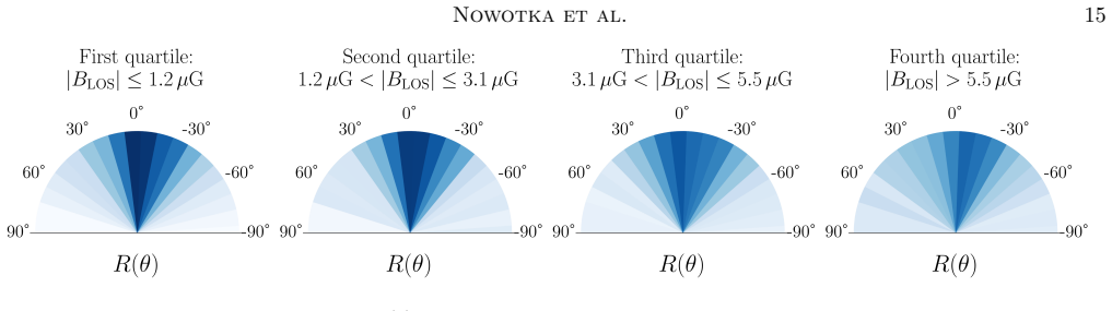
The load-bearing pair is the Zeeman Stokes V fit and the Rolling Hough Transform (RHT), an algorithm that detects coherent linear filaments in maps and assigns each pixel a distribution of orientation angles. From the RHT output the paper constructs Q_HI and U_HI maps, then a circular mean and the circular variance Var(theta_HI), a unitless disorder measure in [0,1] computed over a 2.5-degree patch centered on each background radio source at the absorber's velocity. A 70% emission-dominance criterion (Equation 19) keeps only absorption components that produce most of the cold-neutral-medium emission in the 1.7 km/s channel, so the degree-scale filament statistics can be attributed to gas rel
What would settle it
One test: measure filament orientation dispersion at the absorber's own angular scale (arcminutes rather than degrees) with next-generation HI surveys. The paper finds the correlation only appears at patch sizes of 2.5 degrees and larger; if the trend vanishes at scales matched to the Zeeman pencil beam and to the parsec-scale coherence the paper itself infers, the degree-scale correlation would be a scale-mismatch artifact. A cheaper companion test: re-observe the strongest Zeeman detections (notably the 3C 409 component at B_LOS = 9.1 ± 1.9 microgauss) with doubled integration time and check
Extended reading notes
Core claim
Across 42 spectrally distinct HI absorption components drawn from the Arecibo Millennium Survey and new FAST observations, the magnitude of the line-of-sight magnetic field inferred from Zeeman splitting correlates positively with the circular variance of HI filament orientation angles measured in narrow-channel GALFA-HI emission maps (Spearman rho = 0.3, p = 0.01). The significance is tested against one million null-hypothesis samples that preserve each measurement's uncertainty, with only 1.0–1.4% of simulated samples producing a correlation at least as positive. The signal strengthens when blended components are excluded more aggressively (rho = 0.40, p = 0.004 at an 80% emission-dominanc
Load-bearing premise
The degree-scale filament dispersion (measured over 2.5 degrees, i.e., roughly 4–22 parsecs at the inferred distances) is a faithful statistical picture of the magnetic field seen by the pencil-beam Zeeman absorber at the same velocity; if the filaments trace unrelated gas or a different field-coherence scale, the correlation would be an artifact of line-of-sight structure.
Editorial extensions
If this is right
- If the correlation is real, narrow-channel HI emission morphology becomes a usable statistical tracer of the line-of-sight component of the magnetic field, complementing Zeeman measurements that alone cannot separate field strength from orientation.
- Sight lines dominated by Local Bubble gas show both low |B_LOS| and orderly filaments, implying a field oriented mainly in the plane of the sky there—so inclination effects are already visible in existing data.
- Zeeman absorption components trace fields coherent on parsec scales: co-spectral components within about 7.5 degrees agree in strength and direction (K-S p = 0.002 versus widely separated pairs), with physical separations of a few parsecs inferred from 3D dust maps.
- Sight lines with higher dust extinction and HI column density carry higher average |B_LOS| (Spearman rho = 0.48, p about 0.005), pointing to systematic environmental differences in total field strength or orientation.
- Recovering the total field strength B_TOT from the combination of Zeeman and filament statistics is not yet achieved; the paper identifies larger high-signal-to-noise samples and sharper HI maps as the path forward.
Reading between the lines
- An implication the paper leaves implicit: once calibrated on this sample, the |B_LOS|-versus-disorder slope could be applied across the full GALFA-HI footprint, turning filament statistics in every velocity channel into a map of the field's line-of-sight geometry in regions with no background radio source for Zeeman observations.
- The sharp velocity dependence (weaker at ±6 km/s offsets, gone at ±9 km/s) functions as a built-in consistency check; the editor's reading predicts that spectrally matched, higher-resolution HI data will sharpen the correlation rather than dilute it, because the signal lives in velocity-coherent gas.
- The rise of sight-line-averaged |B_LOS| with dust extinction combined with the absence of a component-level density trend suggests environment, not local cloud density, sets the total field strength; an unstated corollary is that future Zeeman measurements toward CO-dark, low-extinction clouds should come out systematically low.
- The sign disagreement between HI and OH Zeeman measurements toward 3C 133 has an either-or consequence the paper does not pursue: a convention or calibration error would affect cross-tracer Zeeman comparisons broadly, while a real reversal would imply sub-parsec field structure invisible to the paper's few-parsec coherence analysis.
Editorial analysis
A structured set of objections, weighed in public.
Referee Report
Summary. The paper combines Zeeman measurements of HI absorption from the Arecibo Millennium Survey with new FAST observations toward 3C 75, 3C 207, and 3C 409, and uses GALFA-HI narrow-channel emission maps processed with the Rolling Hough Transform to quantify the circular variance of filament orientation angles at the positions and velocities of Zeeman absorbers. In a subsample of 42 spectrally distinct, non-blended components, the authors report a weak positive correlation between |B_LOS| and Var(theta_HI) (Spearman rho = 0.3, p = 0.01), and argue this correlation is robust to RHT parameter choices and angular scale. They also examine the environments probed by the Zeeman measurements using dust extinction, 3D dust maps, OH absorption, and CO emission, and find evidence for parsec-scale coherence of the magnetic field, with most components tracing gas at 100--500 pc, often associated with the Local Bubble wall. The paper interprets the correlation as arising from large-scale variations in magnetic field strength and/or inclination angle across different Galactic environments.
Significance. If the reported correlation is real, it would establish a new velocity-resolved observational link between HI filament morphology and the line-of-sight projection of the magnetic field, with implications for recovering the total magnetic field strength from combined Zeeman and filament measurements. The paper is careful in several respects: it tests RHT parameter choices (Section 5.4), checks robustness to the blending threshold and angular scale, uses null simulations with three different B_TOT distributions, provides new FAST Zeeman data consistent with Arecibo, and combines multi-wavelength environmental diagnostics. These strengths make the central hypothesis worth investigating. However, the headline statistical significance is not yet established because the null model treats the 42 components as independent despite the clustering and coherence demonstrated in the same paper, and because the correlation may be driven by environmental confounders such as A_V and Galactic latitude.
major comments (3)
- [Section 5.3, with Section 7.1] The reported p = 0.01 is computed against a null model (Equations 22--23) that draws 42 independent B_LOS values from the fitted PDF(B_TOT). This independence assumption is inconsistent with the paper's own demonstration in Section 7.1 that Zeeman measurements are coherent within angular separations <= 7.5 deg and velocity separations < 3 km/s. The sample is also strongly clustered, with multiple components per sight line (e.g., five toward 3C 409). Under the null, B_LOS values from the same sight line or nearby sight lines would still be spatially/velocity coherent, so the effective number of independent samples is smaller than 42. The p-value should be recomputed with a cluster-robust permutation or block bootstrap that resamples at the level of sight lines (or coherent angular/velocity neighborhoods) while preserving the pairing of B_LOS with Var(theta_HI). Without this, the central c
- [Section 8.2 and Figure 16] The paper does not test whether the |B_LOS|-Var(theta_HI) correlation survives controlling for environmental variables. Figure 16 shows that the sample splits by A_V and Galactic latitude occupy different regions of the correlation plot, and Section 6.1 reports a significant correlation between A_V (and N_HI) and sight-line averaged |B_LOS|. It is therefore possible that both |B_LOS| and Var(theta_HI) are correlated with a third variable and not directly with each other. A partial Spearman correlation controlling for A_V, N_HI, Galactic latitude, and possibly distance or molecular tracers should be reported. This is important for the physical interpretation: the title and abstract suggest HI filament morphology carries information about B_LOS, but the current analysis does not exclude the possibility that the apparent relationship is an environmental projection.
- [Section 5.1 and 5.3] The selection of the 42 non-blended components uses a 70% dominance threshold in Equation 19, and the paper also reports results for a 0.80 threshold (38 components, rho = 0.40, p = 0.004) and for all 62 usable components (rho = 0.21, p = 0.04). The headline p-value is therefore one of several selection-dependent values, and no correction for this selection or for the multiple tested thresholds is applied. The selection criterion is physically motivated, but the statistical significance should be assessed in a way that accounts for the choice of threshold, or the paper should clearly state that the reported p-values are not adjusted for post-hoc selection. A sensitivity analysis that treats the threshold as a tuning parameter and reports the distribution of p-values across thresholds would be more convincing.
minor comments (5)
- [Section 2.3.3, Eq. (4)] The leakage terms C_on T_on(v) - C_off T_off(v) are not explicitly defined in the text; please define the units and whether C_on/C_off are fitted constants, and briefly explain why the leakage subtraction appears as a difference of two terms.
- [Section 4.3] The definition of circular variance in Eq. (16) uses doubled angles, but the range [0,1] and interpretation as 'disorder' would benefit from a one-sentence clarification that this is the standard axial circular variance.
- [Section 5.4, Figure 8] The text says 'no significant correlation is found at dPOS < 2 deg' while the figure caption says 'dPOS < 2.5 deg'; please unify the notation and the exact angular scale used in the analysis.
- [Section 5.4] The reference to 'Putman et al. (2025, in prep)' should be updated or, if not yet available, flagged as a personal communication with details of the analysis.
- [Section 6.2, Figure 11] The text mentions 'OH 1667 Hz line' in the figure caption; the correct unit is MHz, not Hz. Please correct.
Circularity Check
No significant circularity: the central |BLOS|–Var(θHI) correlation is an empirical result computed from independent datasets, and the fitted null model affects only the conditioning of the p-value, not the correlation itself.
full rationale
The central claim is an empirical Spearman correlation between |BLOS| from HI absorption Zeeman measurements and Var(θHI) from GALFA-HI RHT maps. These two quantities are measured from independent datasets (Stokes V absorption spectra vs. 21-cm emission maps), and the correlation coefficient is computed directly from the observed pairs; it is not generated by any fitted model. The null-hypothesis significance test in §5.3 does fit parameters of PDF(BTOT) (B0=6.2 μG, 9.6 μG; lognormal 1.7/0.2) by maximum likelihood to the same 42 |BLOS| values, but this fit is to the marginal distribution of |BLOS| alone; null samples are then drawn independently of Var(θHI), so the observed ρ is not forced by the fit. The paper also checks three different PDF forms and obtains similar p-values (1.0–1.4%), so the significance is not an artifact of a single fitted ansatz. The more substantive statistical caveat, explicitly acknowledged in §5.2, is that components clustered within one sight line or between nearby sight lines are treated as independent in the null, even though §7.1 demonstrates coherence on scales ≲7.5° and ≲3 km/s. That is a robustness/correctness limitation, not circularity: the correlation coefficient is not defined in terms of the null model, and the null model is not fitted to the joint |BLOS|–Var(θHI) relation. The RHT formalism and the 'HI filaments trace B⊥' premise are cited from prior work including co-author papers (Clark et al. 2014; Clark & Hensley 2019; Halal et al. 2024a), but these are supported by independent starlight-polarization and Planck dust-polarization comparisons and are further tested for parameter sensitivity in this paper; they are not assumed as the target result. No step in the paper reduces by construction to its inputs, and the correlation is not renamed from a known result.
Assumptions & free parameters
free parameters (7)
- B0 (Delta PDF null model) =
6.2 uG
- B0 (Uniform PDF null model) =
9.6 uG
- B0 and sigma (lognormal null model) =
B0=1.7, sigma=0.2
- RHT parameters (DW, theta_FWHM, ZRHT) =
105 arcmin, 5 arcmin, 0.75
- Absorption mask radius per sight line =
3 to 10 arcmin
- Blending threshold =
0.70
- Angular scale dPOS =
2.5 degrees
assumptions (5)
- domain assumption HI filaments trace the plane-of-sky magnetic field orientation
- domain assumption Narrow-channel HI emission near the absorber velocity represents the same cold neutral medium as the absorption component
- domain assumption Magnetic field coherence over the 2.5 degree RHT region
- domain assumption The chosen parametric forms of PDF(BTOT) are representative of the underlying population
- domain assumption Stokes V gradients in the off-source emission are negligible
Cite this review
Pith. "Pith review of Joint Analysis of HI Absorption Zeeman Measurements and the Morphology of Filamentary HI Emission." pith.science (2026). https://pith.science/paper/44NIFT7U
@misc{pith2026250820065,
  author       = {Pith},
  title        = {Pith review of: Joint Analysis of HI Absorption Zeeman Measurements and the Morphology of Filamentary HI Emission},
  year         = {2026},
  howpublished = {\url{https://pith.science/paper/44NIFT7U}},
  note         = {Machine review of arXiv:2508.20065}
}
abstract
We present a joint analysis of HI absorption Zeeman measurements and the morphology of filamentary HI emission to investigate the three-dimensional structure of the magnetic field in the diffuse neutral interstellar medium (ISM). Our analysis is based on the Arecibo Millennium Survey and new data from the Five-hundred-meter Aperture Spherical radio Telescope (FAST) toward radio sources 3C 75, 3C 207, and 3C 409. Toward 3C 409, we make a 4$\sigma$ Zeeman detection and infer $B_{LOS}$ = 9.1 +/- 1.9$\mu$G, in agreement with Arecibo results. We quantify the dispersion of HI filaments at the locations and velocities of Zeeman components using GALFA-HI narrow-channel emission maps. Focusing on a subsample of 42 spectrally distinct components, we find a weak but statistically significant positive correlation (Spearman r = 0.3, $p = 0.01$) between $|B_{LOS}|$ and the circular variance of HI filament orientation angles. To examine its origin, we characterize the environments probed by HI absorption using dust emission, 3D dust maps, OH absorption, and CO emission. We find evidence that existing HI absorption Zeeman measurements trace magnetic fields that are coherent on parsec scales, probe primarily local gas ($100$-$500$ pc, often at distances consistent with the Local Bubble wall), and exhibit systematic differences in the magnitude of $B_{LOS}$. We attribute the correlation between Zeeman measurements and filamentary HI morphology to large-scale variations in magnetic field strength and/or inclination angle across different Galactic environments, which could arise due to the Local Bubble geometry or enhanced total field strength in denser regions.
Figures


Figures from the paper (13 more)




Reference graph
Works this paper leans on
-
[1]
Ade, P. A. R., Ahmed, Z., Amiri, M., et al. 2023, ApJ, 945, 72, doi: 10.3847/1538-4357/acb64c
-
[2]
Alves, M. I. R., Boulanger, F., Ferri` ere, K., & Montier, L. 2018, A&A, 611, L5, doi: 10.1051/0004-6361/201832637
-
[3]
Angarita, Y., Versteeg, M. J. F., Haverkorn, M., et al. 2024, AJ, 168, 47, doi: 10.3847/1538-3881/ad4b14 Astropy Collaboration, Robitaille, T. P., Tollerud, E. J., et al. 2013, A&A, 558, A33, doi: 10.1051/0004-6361/201322068
-
[4]
Beaumont, C. N., Offner, S. S. R., Shetty, R., Glover, S. C. O., & Goodman, A. A. 2013, ApJ, 777, 173, doi: 10.1088/0004-637X/777/2/173
-
[5]
Burkhart, B., Dharmawardena, T. E., Bialy, S., et al. 2025, Nature Astronomy, 9, 1064, doi: 10.1038/s41550-025-02541-7
-
[6]
Cardelli, J. A., Clayton, G. C., & Mathis, J. S. 1989, ApJ, 345, 245, doi: 10.1086/167900
doi:10.1086/167900 1989
-
[7]
2025, AJ, 169, 158, doi: 10.3847/1538-3881/ada8aa
Chen, X., Ching, T.-C., Li, D., et al. 2025, AJ, 169, 158, doi: 10.3847/1538-3881/ada8aa
-
[8]
Ching, T. C., Li, D., Heiles, C., et al. 2022, Nature, 601, 49, doi: 10.1038/s41586-021-04159-x
Show all 85 references
-
[9]
2025, AJ, 170, 116, doi: 10.3847/1538-3881/ade144
Ching, T.-C., Heiles, C., Li, D., et al. 2025, AJ, 170, 116, doi: 10.3847/1538-3881/ade144
2025 doi
-
[10]
Clark, S. E. 2018, ApJL, 857, L10, doi: 10.3847/2041-8213/aabb54
2018 doi
-
[11]
E., & Hensley, B
Clark, S. E., & Hensley, B. S. 2019, ApJ, 887, 136, doi: 10.3847/1538-4357/ab5803
2019 doi
-
[12]
Babler, B. L. 2015, PhRvL, 115, 241302, doi: 10.1103/PhysRevLett.115.241302
2015 doi
-
[13]
E., Peek, J
Clark, S. E., Peek, J. E. G., & Miville-Deschˆ enes, M. A. 2019, ApJ, 874, 171, doi: 10.3847/1538-4357/ab0b3b
2019 doi
-
[14]
E., Peek, J
Clark, S. E., Peek, J. E. G., & Putman, M. E. 2014, ApJ, 789, 82, doi: 10.1088/0004-637X/789/1/82
2014 doi
-
[15]
M., & Kemball, A
Crutcher, R. M., & Kemball, A. J. 2019, Frontiers in Astronomy and Space Sciences, 6, 66, doi: 10.3389/fspas.2019.00066
2019
-
[16]
Troland, T. H. 2010, ApJ, 725, 466, doi: 10.1088/0004-637X/725/1/466
2010 doi
-
[17]
M., & Thaddeus, P
Dame, T. M., & Thaddeus, P. 2022, ApJS, 262, 5, doi: 10.3847/1538-4365/ac7e53
2022 doi
-
[18]
2024, A&A, 685, A82, doi: 10.1051/0004-6361/202347628
Edenhofer, G., Zucker, C., Frank, P., et al. 2024, A&A, 685, A82, doi: 10.1051/0004-6361/202347628
2024 doi
-
[19]
1991, An Introduction to Probability Theory and Its Applications, Volume 2 (John Wiley & Sons)
Feller, W. 1991, An Introduction to Probability Theory and Its Applications, Volume 2 (John Wiley & Sons)
1991
-
[20]
Field, G. B. 1958, Proceedings of the IRE, 46, 240, doi: 10.1109/JRPROC.1958.286741
1958
-
[21]
M., Ade, P
Fissel, L. M., Ade, P. A. R., Angil` e, F. E., et al. 2019, ApJ, 878, 110, doi: 10.3847/1538-4357/ab1eb0
2019 doi
-
[22]
Garrett, J. D. 2021, None, doi: 10.5281/zenodo.4106649
2021 doi
- [23]
-
[24]
Green, G. M. 2018, The Journal of Open Source Software, 3, 695, doi: 10.21105/joss.00695
2018 doi
-
[25]
E., Cukierman, A., Beck, D., & Kuo, C.-L
Halal, G., Clark, S. E., Cukierman, A., Beck, D., & Kuo, C.-L. 2024a, ApJ, 961, 29, doi: 10.3847/1538-4357/ad06aa
-
[26]
E., & Tahani, M
Halal, G., Clark, S. E., & Tahani, M. 2024b, ApJ, 973, 54, doi: 10.3847/1538-4357/ad61e0
-
[27]
Han, J. L. 2017, ARA&A, 55, 111, doi: 10.1146/annurev-astro-091916-055221
2017 doi
-
[28]
R., Millman, K
Harris, C. R., Millman, K. J., van der Walt, S. J., et al. 2020, Nature, 585, 357, doi: 10.1038/s41586-020-2649-2
2020 doi
-
[29]
1989, ApJ, 336, 808, doi: 10.1086/167051
Heiles, C. 1989, ApJ, 336, 808, doi: 10.1086/167051
1989 doi
-
[30]
A., McKee, C
Heiles, C., Goodman, A. A., McKee, C. F., & Zweibel, E. G. 1993, in Protostars and Planets III, ed. E. H. Levy & J. I. Lunine, 279
1993
-
[31]
Heiles, C., & Troland, T. H. 2003, ApJS, 145, 329, doi: 10.1086/367785
2003 doi
-
[32]
Heiles, C., & Troland, T. H. 2004, ApJS, 151, 271, doi: 10.1086/381753
2004 doi
-
[33]
Heiles, C., & Troland, T. H. 2005, ApJ, 624, 773, doi: 10.1086/428896
2005 doi
-
[34]
2001, PASP, 113, 1247, doi: 10.1086/323290
Heiles, C., Perillat, P., Nolan, M., et al. 2001, PASP, 113, 1247, doi: 10.1086/323290
2001 doi
-
[35]
S., Zhang, C., & Bock, J
Hensley, B. S., Zhang, C., & Bock, J. J. 2019, ApJ, 887, 159, doi: 10.3847/1538-4357/ab5183 HI4PI Collaboration, Ben Bekhti, N., Fl¨ oer, L., et al. 2016, A&A, 594, A116, doi: 10.1051/0004-6361/201629178
2019 doi
-
[36]
D., & Krumholz, M
Hu, Z., Wibking, B. D., & Krumholz, M. R. 2023, MNRAS, 521, 5604, doi: 10.1093/mnras/stad931
2023 doi
-
[37]
Hunter, J. D. 2007, Computing in Science & Engineering, 9, 90, doi: 10.1109/MCSE.2007.55
2007 doi
-
[38]
2020, ApJ, 890, 153, doi: 10.3847/1538-4357/ab672b
Jiang, H., Li, H.-b., & Fan, X. 2020, ApJ, 890, 153, doi: 10.3847/1538-4357/ab672b
2020 doi
-
[39]
2019, Science China
Jiang, P., Yue, Y., Gan, H., et al. 2019, Science China
2019
-
[40]
Physics, Mechanics, and Astronomy, 62, 959502, doi: 10.1007/s11433-018-9376-1
-
[41]
2020, Research in Astronomy and Astrophysics, 20, 064, doi: 10.1088/1674-4527/20/5/64
Jiang, P., Tang, N.-Y., Hou, L.-G., et al. 2020, Research in Astronomy and Astrophysics, 20, 064, doi: 10.1088/1674-4527/20/5/64
2020 doi
-
[42]
Kalberla, P. M. W., Kerp, J., & Haud, U. 2020, A&A, 639, A26, doi: 10.1051/0004-6361/202037602
2020 doi
-
[43]
Kalberla, P. M. W., Kerp, J., Haud, U., et al. 2016, ApJ, 821, 117, doi: 10.3847/0004-637X/821/2/117 Nowotka et al. 25
2016 doi
- [44]
-
[45]
A., et al
Lee, M.-Y., Stanimirovi´ c, S., Douglas, K. A., et al. 2012, ApJ, 748, 75, doi: 10.1088/0004-637X/748/2/75
2012 doi
-
[46]
Lei, M., & Clark, S. E. 2023, ApJ, 947, 74, doi: 10.3847/1538-4357/acc02a
2023 doi
-
[47]
S., & Dor´ e, O
Lenz, D., Hensley, B. S., & Dor´ e, O. 2017, ApJ, 846, 38, doi: 10.3847/1538-4357/aa84af
2017 doi
-
[48]
2018a, IEEE Microwave Magazine, 19, 112, doi: 10.1109/MMM.2018.2802178
Li, D., Wang, P., Qian, L., et al. 2018a, IEEE Microwave Magazine, 19, 112, doi: 10.1109/MMM.2018.2802178
2018
-
[49]
2018b, ApJS, 235, 1, doi: 10.3847/1538-4365/aaa762
Li, D., Tang, N., Nguyen, H., et al. 2018b, ApJS, 235, 1, doi: 10.3847/1538-4365/aaa762
-
[50]
R., Vera-Ciro, C., Murray, C
Lindner, R. R., Vera-Ciro, C., Murray, C. E., et al. 2015, AJ, 149, 138, doi: 10.1088/0004-6256/149/4/138
2015 doi
-
[51]
2001, A&A, 371, 698, doi: 10.1051/0004-6361:20010395
Liszt, H. 2001, A&A, 371, 698, doi: 10.1051/0004-6361:20010395
2001 doi
-
[52]
2016, MNRAS, 460, 1934, doi: 10.1093/mnras/stw1061
Malinen, J., Montier, L., Montillaud, J., et al. 2016, MNRAS, 460, 1934, doi: 10.1093/mnras/stw1061
2016 doi
-
[53]
G., Blagrave, K
Martin, P. G., Blagrave, K. P. M., Lockman, F. J., et al. 2015, ApJ, 809, 153, doi: 10.1088/0004-637X/809/2/153
2015 doi
-
[54]
A., & Troland, T
Mayo, E. A., & Troland, T. H. 2012, AJ, 143, 32, doi: 10.1088/0004-6256/143/2/32
2012 doi
- [55]
- [56]
-
[57]
E., Peek, J
Murray, C. E., Peek, J. E. G., & Kim, C.-G. 2020, ApJ, 899, 15, doi: 10.3847/1538-4357/aba19b
2020 doi
-
[58]
E., Stanimirovi´ c, S., Goss, W
Murray, C. E., Stanimirovi´ c, S., Goss, W. M., et al. 2018, ApJS, 238, 14, doi: 10.3847/1538-4365/aad81a
2018 doi
-
[59]
C., Goodman, A
Myers, P. C., Goodman, A. A., Gusten, R., & Heiles, C. 1995, ApJ, 442, 177, doi: 10.1086/175433
1995 doi
-
[60]
R., Miville-Deschˆ enes, M
Nguyen, H., Dawson, J. R., Miville-Deschˆ enes, M. A., et al. 2018, ApJ, 862, 49, doi: 10.3847/1538-4357/aac82b O’Neill, T. J., Goodman, A. A., Soler, J. D., Zucker, C., &
2018 doi
-
[61]
Han, J. J. 2025, ApJ, 988, 191, doi: 10.3847/1538-4357/ade306 O’Neill, T. J., Zucker, C., Goodman, A. A., & Edenhofer, G. 2024, ApJ, 973, 136, doi: 10.3847/1538-4357/ad61de OpenAI. 2022, Introducing ChatGPT,, https://openai.com/blog/chatgpt Pandas Development Team. 2020, None,...
2025 doi
-
[62]
Peek, J. E. G., & Clark, S. E. 2019, ApJL, 886, L13, doi: 10.3847/2041-8213/ab53de
2019 doi
-
[63]
Peek, J. E. G., Babler, B. L., Zheng, Y., et al. 2018, ApJS, 234, 2, doi: 10.3847/1538-4365/aa91d3 Planck Collaboration, Ade, P. A. R., Aghanim, N., et al. 2015, A&A, 576, A105, doi: 10.1051/0004-6361/201424086 Planck Collaboration, Ade, P. A. R., Aghanim, N., et al. 2016a, A&...
2018 doi
-
[64]
2020, The Innovation, 1, 100053, doi: 10.1016/j.xinn.2020.100053
Qian, L., Yao, R., Sun, J., et al. 2020, The Innovation, 1, 100053, doi: 10.1016/j.xinn.2020.100053
2020
-
[65]
2011, MNRAS, 418, 467, doi: 10.1111/j.1365-2966.2011.19497.x
Remazeilles, M., Delabrouille, J., & Cardoso, J.-F. 2011, MNRAS, 418, 467, doi: 10.1111/j.1365-2966.2011.19497.x
2011
-
[66]
2008, PhD thesis, University of California, Berkeley
Robishaw, T. 2008, PhD thesis, University of California, Berkeley
2008
-
[67]
2021, in The WSPC Handbook of Astronomical Instrumentation, Volume 1: Radio Astronomical Instrumentation, ed
Robishaw, T., & Heiles, C. 2021, in The WSPC Handbook of Astronomical Instrumentation, Volume 1: Radio Astronomical Instrumentation, ed. A. Wolszczan, 127–158, doi: 10.1142/9789811203770 0006
2021 doi
-
[68]
P., Troland, T
Sarma, A. P., Troland, T. H., Roberts, D. A., & Crutcher, R. M. 2000, ApJ, 533, 271, doi: 10.1086/308667
2000 doi
-
[69]
P., Troland, T
Sarma, A. P., Troland, T. H., & Rupen, M. P. 2002, ApJ, 564, 696, doi: 10.1086/324234
2002 doi
-
[70]
J., Killeen, N
Sault, R. J., Killeen, N. E. B., Zmuidzinas, J., & Loushin, R. 1990, ApJS, 74, 437, doi: 10.1086/191505
1990 doi
-
[71]
J., Burkhart, B., et al
Saxena, S., Haworth, T. J., Burkhart, B., et al. 2025, MNRAS, 540, L109, doi: 10.1093/mnrasl/slaf044
2025 doi
-
[72]
Seta, A., & McClure-Griffiths, N. M. 2025, MNRAS, 539, 1024, doi: 10.1093/mnras/staf520
2025 doi
-
[73]
D., Bracco, A., & Pon, A
Soler, J. D., Bracco, A., & Pon, A. 2018, A&A, 609, L3, doi: 10.1051/0004-6361/201732203
2018 doi
-
[74]
D., Beuther, H., Rugel, M., et al
Soler, J. D., Beuther, H., Rugel, M., et al. 2019, A&A, 622, A166, doi: 10.1051/0004-6361/201834300
2019 doi
-
[75]
R., Moran, J
Thompson, A. R., Moran, J. M., & Swenson, Jr., G. W. 2017, Interferometry and Synthesis in Radio Astronomy, 3rd Edition, doi: 10.1007/978-3-319-44431-4
2017 doi
-
[76]
L., Troland, T
Thompson, K. L., Troland, T. H., & Heiles, C. 2019, ApJ, 884, 49, doi: 10.3847/1538-4357/ab364e
2019 doi
-
[77]
V., Mouschovias, T
Tritsis, A., Panopoulou, G. V., Mouschovias, T. C., Tassis, K., & Pavlidou, V. 2015, MNRAS, 451, 4384, doi: 10.1093/mnras/stv1133
2015 doi
-
[78]
H., & Heiles, C
Troland, T. H., & Heiles, C. 1982, ApJ, 252, 179, doi: 10.1086/159544 van der Velden, E. 2020, The Journal of Open Source Software, 5, 2004, doi: 10.21105/joss.02004
1982 doi
-
[79]
Verschuur, G. L. 1968, PhRvL, 21, 775, doi: 10.1103/PhysRevLett.21.775
1968 doi
-
[80]
E., et al
Virtanen, P., Gommers, R., Oliphant, T. E., et al. 2020, Nature Methods, 17, 261, doi: 10.1038/s41592-019-0686-2 26 Nowotka et al
2020 doi
-
[81]
Waskom, M. L. 2021, Journal of Open Source Software, 6, 3021, doi: 10.21105/joss.03021
2021 doi
-
[82]
J., Srinivasan, S., Pudritz, R
Whitworth, D. J., Srinivasan, S., Pudritz, R. E., et al. 2025, MNRAS, 540, 2762, doi: 10.1093/mnras/staf901
2025 doi
-
[83]
W., Jefferts, K
Wilson, R. W., Jefferts, K. B., & Penzias, A. A. 1970, ApJL, 161, L43, doi: 10.1086/180567
1970 doi
-
[84]
M., & Rix, H.-W
Zhang, X., Green, G. M., & Rix, H.-W. 2023, MNRAS, 524, 1855, doi: 10.1093/mnras/stad1941
2023 doi
-
[85]
2019, The Journal of Open Source Software, 4, 1298, doi: 10.21105/joss.01298
Zonca, A., Singer, L., Lenz, D., et al. 2019, The Journal of Open Source Software, 4, 1298, doi: 10.21105/joss.01298
2019 doi
Reviewed August 5, 2026 · model on record in the stance chip above.
Discussion (0). Continue with ORCID to comment.