REVIEW 3 major objections 4 minor 54 references
Testing tidal theory using Gaia binaries: the red giant branch
T0 review · 3 major / 4 minor · reviewed 2026-08-10 · deepseek-v4-flash
Pith's one-line read Gaia red-giant binaries stay circular twice as far out as f-mode tidal theory allows, pointing to an extra circularization process in the early red giant branch.
desk verdict A genuinely new forward-model test of tidal circularization against 30,000 Gaia giants; the early-RGB discrepancy is real but its size is not yet secure because it sits on the adopted eddy-viscosity prescription. read the letter →
The pith
A machine-rendered reading of the paper's core claim, the machinery that carries it, and where it could break.
The reading
What carries the argument
The central machinery is the 'f-mode' tidal model: the tidal response of the evolving 1.5-solar-mass primary is expanded in the star's fundamental and lowest-order pressure modes, and each mode's dissipation is evaluated with a frequency-dependent eddy viscosity from convective turbulence. The resulting dissipative coefficients $\kappa_{mk}$ enter secular equations for orbital decay, eccentricity damping, and spin evolution that are integrated along the stellar evolutionary track. The organizing diagnostic is the dimensionless ratio $a/R$, with $\beta \equiv a(1-e)/R$ marking the eccentricity upper envelope; plotting eccentricity against $a/R$ makes both theory and data nearly stationary across evolutionary stages, so the gap between the predicted boundary at $a/R \approx 4$ and the observed early-RGB reach at $\beta \approx 6$ becomes the measurable quantity that drives the conclusion.
What would settle it
Compute the early-RGB population with an eddy-viscosity prescription that omits or weakens the fast-tide suppression in Equation (7); if the predicted circularization boundary shifts from $a/R \approx 4$ to $\beta \approx 6$, the claimed need for an additional circularization process would not be supported.
Extended reading notes
Core claim
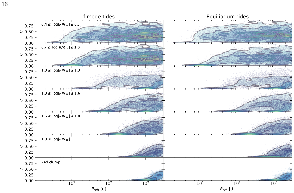
On its own terms, this paper claims that f-mode tidal theory with a frequency-dependent eddy viscosity predicts a universal circularization boundary of $a/R \approx 4$ for red giants, independent of the star's position on the red giant branch. Against that prediction, Gaia binaries in the early red giant phase are observed circularized out to $\beta \approx 6$ and show an extended cool island of circular orbits out to $a/R \sim 10$--$15$, about twice the theoretical reach; in the late red giant branch the observed reach shrinks to $\beta \approx 3$ and agrees with the model. From this the authors conclude that an additional circularization process must act in the early red giant branch, and they note the same missing physics may underlie the even larger discrepancy long seen for main-sequence binaries. The calculations also produce two by-products: tides can spin giant primaries up to rotation rates that should change their mass loss, and many binaries may enter Roche-lobe overflow while still significantly eccentric.
Load-bearing premise
The predicted circularization limit rests on the assumed eddy-viscosity prescription for convective envelopes, and if the true viscosity is stronger than the fast-tide suppression allows, the theory's boundary would move outward and the early-red-giant discrepancy would shrink or vanish.
Editorial extensions
If this is right
- If the f-mode limit is fixed at $a/R \approx 4$, every red-giant binary with dimensionless pericenter $\beta \lesssim 4$ should be effectively circular; the early-RGB binaries with $\beta \approx 6$ mark where that rule fails.
- Tidal spin-up can bring close giant primaries near orbital synchronization, roughly $\Omega/\omega_{\rm dyn} \approx 0.3$ at Roche-lobe overflow for a 2/3 mass ratio, so mass-loss prescriptions based on slowly rotating single stars need revision for these binaries.
- Binaries with initial periods near $10^3$ to $3\times 10^3$ days can begin Roche-lobe overflow while still substantially eccentric, contradicting older equilibrium-tide expectations of full circularization beforehand.
- If the early-RGB excess is real, it may share a mechanism with the main-sequence cool island, turning two separate tidal-theory failures into one missing-process problem.
Reading between the lines
- A direct test would be to rerun the population calculation with a weaker fast-tide suppression in the eddy-viscosity law; if the predicted boundary moves from $a/R \approx 4$ to $\approx 6$ in the early RGB, the claimed missing process would dissolve.
- Because the model predicts a universal $a/R$ limit, observed circularization periods should scale linearly with primary radius; future samples with asteroseismic radii can test this scaling and separate radius errors from genuine tidal effects.
- The early-RGB excess could come from internal gravity waves breaking in the still-substantial radiative core, so comparing same-radius giants of different masses (hence different core sizes) could discriminate among the proposed mechanisms.
- Tidal spin-up out to periods of roughly 5000 days on the RGB and 10,000 days on the AGB should be measurable in asteroseismic rotation rates of red giants, providing an independent check of the dissipation model.
Editorial analysis
A structured set of objections, weighed in public.
Referee Report
Summary. The paper confronts state-of-the-art tidal theory with the Gaia DR3 sample of ~31,500 red-giant binaries. The authors build a forward model: a 1.5 M⊙ primary (with a 1.0 M⊙ companion) is evolved through the RGB and AGB in MESA; linear tidal responses are computed in an f-mode/p-mode eigenmode expansion (and in a zero-frequency 'equilibrium' variant) using GYRE; dissipation is supplied by a frequency-dependent eddy-viscosity model (Eq. 7) calibrated to the local simulations of Duguid et al. (2020); and a synthetic population is generated from observationally motivated initial period and eccentricity distributions (Section 4.3). The model predicts that the eccentricity upper envelope in a/R space is pinned at β ≡ a(1−e)/R ≈ 4 at every RGB stage. The Gaia data instead show an envelope that starts at β ≈ 6 in the early RGB and declines to β ≈ 3 near the tip, plus 'cool islands' of circular orbits extending to a/R ≈ 10–15 in early stages, about twice the predicted reach. The paper concludes that f-mode tides with the adopted viscous prescription describe the late RGB well but that 'an additional circularization process' is needed during the early RGB. It also reports theory-driven predictions of strong tidal spin-up of giant primaries (with consequences for mass loss) and of binaries beginning Roche-lobe overflow while still significantly eccentric.
Significance. If substantiated, the early-RGB discrepancy is a significant result: it connects the long-standing main-sequence tidal-circularization problem to evolved stars and points to missing dissipation physics (internal gravity waves, inertial waves, mode locking, or magnetic effects) in early-RGB convective envelopes. The paper's method is a genuine strength: the predicted a/R ≈ 4 boundary is produced from first principles (a linear f-mode response plus an eddy viscosity from independent local simulations), with no parameter fitted to the Gaia circularization data, and the a/R rescaling makes the comparison clean and physically motivated. The paper also makes concrete, falsifiable predictions: spin-up to Ω/ω_dyn ≈ 0.3 at RLOF, eccentric RLOF onset, and synchronization out to ~5000-day periods on the RGB. The main weakness is identified by the authors themselves: Section 5 notes that the adopted viscosity prescription 'may be too conservative,' and the early-RGB discrepancy is concentrated precisely in the regime where the uncertain fast-tide suppression branch of Eq. (7) acts (short-period orbits, with ω/ω_c ≳ 1–5 in parts of the envelope).
major comments (3)
- [§3.3, Eq. (7); §5; §6] The central quantitative claim — that f-mode tides plus the adopted eddy viscosity cap tidal circularization at a/R ≈ 4 on the entire RGB, and hence that 'there needs to be an additional circularization process during the early RGB' (Section 6) — depends on the high-frequency branch of the viscosity prescription in Eq. (7). The early-RGB binaries at issue have the shortest orbital periods (Fig. 4), so their tidal frequencies place a significant fraction of the convective envelope in the frequency-dependent suppressed regimes (1 ≲ ω/ω_c ≲ 5 in the middle branch and ≳ 5 in the fast branch), including deeper zones at the largest ratios. Section 5 concedes both that the Duguid et al. (2020) scaling suppresses dissipation 'stronger in the early RGB' and that the adopted prescription 'may be too conservative.' Since the comparison in Fig. 11 is a factor-of-two mismatch in exactly this regime, the manuscript should include a sensitivity study in which the predicted β and cool-island edges are recomputed for the plausible range of viscosity scalings (e.g., Zahn (1977) without high-frequency suppression, the Goldreich & Nicholson (1977) form with varied prefactor, and the alternatives of Goodman & Oh (1997) and Terquem (2021, 2023)), and the resulting change in the predicted boundary should be reported. Absent this test, the discrepancy that motivates the paper's main conclusion is not established.
- [§2.2, Figs. 4 and 11] The measured quantities used for the discrepancy claim — the upper-envelope values β ≈ 6.5 → 3.0 and the cool-island edges at a/R ≈ 10–15 (Fig. 4, right panels) — are reported without uncertainties. Section 2.2 states that these uncertainties 'are hard to quantify at this moment,' but the central result is precisely a comparison of these numbers with the theoretical β ≈ 4 boundary (Fig. 11). To support a factor-of-two claim, the paper should provide at least a bootstrap estimate of the sampling uncertainty in β and the island edges (e.g., resampling the binary catalog), propagate the quoted 2–4% eccentricity errors, and test the sensitivity of the derived β values to the adopted Gaia masses in the period-to-a/R conversion. Without error bars on the observational limits, the statistical significance of the early-RGB discrepancy cannot be assessed.
- [§2.2 vs. §3.1; Fig. 10] The two sides of the comparison use inconsistent mass assumptions. Observed a/R values are computed with a total mass of 1.5× the Gaia primary mass (Section 2.2), while the theoretical population is evolved with M + M′ = 2.5 M⊙ for a 1.5 M⊙ primary, i.e., 1.67× (Section 3.1); this produces a ~4% systematic offset in a/R between data and model. In addition, the model uses a single 1.5 M⊙ track while the observed sample spans roughly 1–10 M⊙ (Fig. 3); the claim in Section 3.1 that radius rather than mass controls the tidal evolution is plausible but untested. Computing even one additional track (e.g., 1.0 M⊙ and 2.5 M⊙ primaries) would show whether the predicted a/R ≈ 4 boundary is robust to the primary mass. These checks are inexpensive and directly bear on the quality of the comparison in Fig. 10.
minor comments (4)
- [Appendix B, text after Eq. (B5)] The boundary-conditions sentence contains a duplicated phrase: 'that the normal and that the normal and tangential stresses vanish'; it should read 'that the normal and tangential stresses vanish.'
- [Fig. 1 caption] The label '1.5M' on the evolutionary track should read '1.5 M⊙' in both the caption and the figure legend.
- [§2.2, red-clump excision] The red-clump excision combines a density-peak criterion with a P < 300 day cut; a brief statement of how the derived β values and cool-island edges change when this cut is varied (e.g., 200 or 400 days) would strengthen confidence in the sample boundary.
- [Software and data availability] The text lists the software packages used (MESA, GYRE, scipy, numpy) but does not state where the MESA tracks, pre-computed mode properties, or the orbital-integration code can be obtained; making these available would substantially aid reproducibility of the population-level predictions in Figs. 10 and 12.
Circularity Check
No significant circularity: the predicted a/R≈4 boundary is computed from an independently sourced eddy-viscosity model and a linear f-mode tidal response, not fitted to the Gaia giant binaries.
full rationale
The predicted circularization boundary a/R ≈ 4 is produced by integrating the secular tidal equations (10)-(13) with dissipation coefficients κ_mk computed from the linear f-mode response (Appendix B, Eq. B7) and the eddy-viscosity law in Eq. (7), which is adopted from Duguid et al. (2020) local simulations. No parameter in that chain is fitted to the ~30,000 Gaia giant binaries; the observed β ≡ a(1−e)/R values in Figs. 4 and 10 are an independent comparison set. The initial eccentricity distribution (Rayleigh, σ_e ≈ 0.30) is cited to the authors' own Wu et al. (2024), but it is a prior empirical measurement from wide/main-sequence Gaia binaries, not derived from the target red-giant circularization envelope, so it is not a fitted input renamed as a prediction. The paper itself flags the main sensitivity in Section 5: 'It is possible that we have adopted a prescription for turbulent viscosity that is too conservative.' That is a model-uncertainty caveat, not a circular reduction: the predicted a/R limit is contingent on a physical input sourced independently of the data being predicted. The total-mass assumption for period-to-a/R conversion is a systematic uncertainty, not a definitional shortcut. No equation in the paper reduces to its own input by construction, and the discrepancy (predicted β≈4 vs observed early-RGB β≈6) is a genuine forward-model comparison.
Assumptions & free parameters
free parameters (4)
- Eddy viscosity scaling coefficients =
5, 1/2, 25*sqrt(20); thresholds |ω|/ωc = 10^-2 and 5
- Initial stellar rotation rate =
Ω = 0.01 ω_dyn
- Total system mass multiplier =
1.5 × primary mass
- Initial period and eccentricity distribution parameters =
log-normal mean 5, σ=2.3; Rayleigh σ_e=0.30
assumptions (9)
- domain assumption The tidal response can be represented by a truncated expansion in the f-mode and ten lowest-order p-modes
- domain assumption The inner boundary of the tidal calculation is set at the outer edge of the radiative core
- domain assumption Primary stars rotate rigidly and uniformly
- domain assumption Initial eccentricities follow a Rayleigh distribution with σ_e = 0.30, independent of period
- domain assumption Mass loss follows the Reimers/Blöcker prescriptions and is not modified by tidal spin-up
- domain assumption Roche-lobe overflow does not significantly alter tidal evolution before integration is halted
- standard math The linearized tidal response equations (2)-(5) are valid
- domain assumption Gaia DR3 astrophysical parameters (radii, masses) are sufficiently accurate for the a/R conversion
- domain assumption A single 1.5 M_sun primary evolutionary track represents all observed RGB primaries
Cite this review
Pith. "Pith review of Testing tidal theory using Gaia binaries: the red giant branch." pith.science (2026). https://pith.science/paper/46QEJGTQ
@misc{pith2026250113929,
  author       = {Pith},
  title        = {Pith review of: Testing tidal theory using Gaia binaries: the red giant branch},
  year         = {2026},
  howpublished = {\url{https://pith.science/paper/46QEJGTQ}},
  note         = {Machine review of arXiv:2501.13929}
}
read the original abstract
Tidal interaction is a major ingredient in the theory of binary evolution. Here, we study tidal circularization in binaries with red giant primaries. We compute the tidal evolution for binaries as their primary stars evolve along the red giant branch, under dissipation of dynamical tides in the convective envelope. We then compare this evolution with a sample of ~30,000 red giant binaries reported by Gaia DR3. These binaries clearly show the expected gradual advance of tidal circularization, as the primary expands. But some tension with theory remains. While our calculations always predict a critical separation for tidal circularization at about 3-4 times the stellar radii, binaries with less evolved giants are observed to be circularized out to about twice as far. They also exhibit an overly extended `cool island', a collection of circular orbits that reach a couple times beyond the circularization limit. These discrepancies are reminiscent of, but less severe than, the situation for main-sequence binaries. We also find that tides can spin giant stars up to rotation rates that should affect their mass-loss. Additionally, many binaries may begin mass transfer while still eccentric.
Figures


Figures from the paper (8 more)


Reference graph
Works this paper leans on
-
[1]
Barker, A. J. 2022, ApJL, 927, L36, doi: 10.3847/2041-8213/ac5b63
-
[2]
Barker, A. J., & Astoul, A. A. V. 2021, MNRAS, 506, L69, doi: 10.1093/mnrasl/slab077
-
[3]
2023, MNRAS, 522, 1184, doi: 10.1093/mnras/stad999
Bashi, D., Mazeh, T., & Faigler, S. 2023, MNRAS, 522, 1184, doi: 10.1093/mnras/stad999
-
[4]
G., Mathis, S., Gallet, F., et al
Beck, P. G., Mathis, S., Gallet, F., et al. 2018, MNRAS, 479, L123, doi: 10.1093/mnrasl/sly114
-
[5]
Beck, P. G., Grossmann, D. H., Steinwender, L., et al. 2024, A&A, 682, A7, doi: 10.1051/0004-6361/202346810 Bl¨ ocker, T. 1995, A&A, 297, 727
-
[6]
Braviner, H. J., & Ogilvie, G. I. 2015, MNRAS, 447, 1141, doi: 10.1093/mnras/stu2521
-
[7]
2012, MNRAS, 427, 127, doi: 10.1111/j.1365-2966.2012.21948.x
Bressan, A., Marigo, P., Girardi, L., et al. 2012, MNRAS, 427, 127, doi: 10.1111/j.1365-2966.2012.21948.x
arXiv 2012
-
[8]
Townsend, R. H. D. 2024, Nature Astronomy, 8, 1387, doi: 10.1038/s41550-024-02351-3
Show all 54 references
-
[9]
D., Barker, A
Duguid, C. D., Barker, A. J., & Jones, C. A. 2020, MNRAS, 497, 3400, doi: 10.1093/mnras/staa2216
2020 doi
-
[10]
D., de Vries, N
Duguid, C. D., de Vries, N. B., Lecoanet, D., & Barker, A. J. 2024, ApJL, 966, L14, doi: 10.3847/2041-8213/ad3c40
2024 doi
-
[11]
Eggleton, P. P. 1983, ApJ, 268, 368, doi: 10.1086/160960
1983 doi
- [12]
-
[13]
2017, MNRAS, 472, 1538, doi: 10.1093/mnras/stx2135 Gaia Collaboration, Arenou, F., Babusiaux, C., et al
Fuller, J. 2017, MNRAS, 472, 1538, doi: 10.1093/mnras/stx2135 Gaia Collaboration, Arenou, F., Babusiaux, C., et al. 2023, A&A, 674, A34, doi: 10.1051/0004-6361/202243782
2017 doi
-
[14]
Goldreich, P., & Nicholson, P. D. 1977, Icarus, 30, 301, doi: 10.1016/0019-1035(77)90163-4
1977 doi
-
[15]
Goodman, J., & Dickson, E. S. 1998, ApJ, 507, 938, doi: 10.1086/306348
1998 doi
-
[16]
Goodman, J., & Oh, S. P. 1997, ApJ, 486, 403, doi: 10.1086/304505
1997 doi
-
[17]
I., & Barker, A
Guo, Z., Ogilvie, G. I., & Barker, A. J. 2023, MNRAS, 521, 1353, doi: 10.1093/mnras/stad569
2023 doi
-
[18]
2020, Research in Astronomy and Astrophysics, 20, 161, doi: 10.1088/1674-4527/20/10/161
Han, Z.-W., Ge, H.-W., Chen, X.-F., & Chen, H.-L. 2020, Research in Astronomy and Astrophysics, 20, 161, doi: 10.1088/1674-4527/20/10/161
2020 doi
-
[19]
R., Millman, K
Harris, C. R., Millman, K. J., van der Walt, S. J., et al. 2020, Nature, 585, 357, doi: 10.1038/s41586-020-2649-2
2020 doi
-
[20]
Hunter, J. D. 2007, Computing in Science & Engineering, 9, 90, doi: 10.1109/MCSE.2007.55
2007 doi
-
[21]
R., Tout, C
Hurley, J. R., Tout, C. A., & Pols, O. R. 2002, MNRAS, 329, 897, doi: 10.1046/j.1365-8711.2002.05038.x
2002
-
[22]
S., Bauer, E
Jermyn, A. S., Bauer, E. B., Schwab, J., et al. 2023, ApJS, 265, 15, doi: 10.3847/1538-4365/acae8d
2023 doi
-
[23]
2010, A&A, 516, A64, doi: 10.1051/0004-6361/201014337
Leconte, J., Chabrier, G., Baraffe, I., & Levrard, B. 2010, A&A, 516, A64, doi: 10.1051/0004-6361/201014337
2010 doi
-
[24]
Lin, Y., & Ogilvie, G. I. 2018, MNRAS, 474, 1644, doi: 10.1093/mnras/stx2764
2018 doi
-
[25]
2008, in EAS Publications Series, Vol
Mazeh, T. 2008, in EAS Publications Series, Vol. 29, Tidal Effects in Stars, Planets and Disks, ed. M. J. Goupil & J. P. Zahn, 1–65, doi: 10.1051/eas:0829001
2008 doi
-
[26]
Meibom, S., & Mathieu, R. D. 2005, ApJ, 620, 970, doi: 10.1086/427082
2005 doi
-
[27]
D., & Stassun, K
Meibom, S., Mathieu, R. D., & Stassun, K. G. 2006, ApJ, 653, 621, doi: 10.1086/508252
2006 doi
-
[28]
2017, ApJS, 230, 15, doi: 10.3847/1538-4365/aa6fb6
Moe, M., & Di Stefano, R. 2017, ApJS, 230, 15, doi: 10.3847/1538-4365/aa6fb6
2017 doi
-
[29]
2023, A&A, 674, A16, doi: 10.1051/0004-6361/202245330
Mowlavi, N., Holl, B., Lecoeur-Ta ¨ ıbi, I., et al. 2023, A&A, 674, A16, doi: 10.1051/0004-6361/202245330
2023 doi
-
[30]
Ogilvie, G. I. 2013, MNRAS, 429, 613, doi: 10.1093/mnras/sts362 —. 2014, ARA&A, 52, 171, doi: 10.1146/annurev-astro-081913-035941
2013 doi
- [31]
-
[32]
2011, ApJS, 192, 3, doi: 10.1088/0067-0049/192/1/3
Paxton, B., Bildsten, L., Dotter, A., et al. 2011, ApJS, 192, 3, doi: 10.1088/0067-0049/192/1/3
2011 doi
-
[33]
2013, ApJS, 208, 4, doi: 10.1088/0067-0049/208/1/4
Paxton, B., Cantiello, M., Arras, P., et al. 2013, ApJS, 208, 4, doi: 10.1088/0067-0049/208/1/4
2013 doi
-
[34]
2015, ApJS, 220, 15, doi: 10.1088/0067-0049/220/1/15
Paxton, B., Marchant, P., Schwab, J., et al. 2015, ApJS, 220, 15, doi: 10.1088/0067-0049/220/1/15
2015 doi
-
[35]
B., et al
Paxton, B., Schwab, J., Bauer, E. B., et al. 2018, ApJS, 234, 34, doi: 10.3847/1538-4365/aaa5a8
2018 doi
-
[36]
2019, ApJS, 243, 10, doi: 10.3847/1538-4365/ab2241
Paxton, B., Smolec, R., Schwab, J., et al. 2019, ApJS, 243, 10, doi: 10.3847/1538-4365/ab2241
2019 doi
-
[37]
2007, in SF2A-2007: Proceedings of the Annual meeting of the French Society of Astronomy and Astrophysics, ed
Pichon, B. 2007, in SF2A-2007: Proceedings of the Annual meeting of the French Society of Astronomy and Astrophysics, ed. J. Bouvier, A. Chalabaev, & C. Charbonnel, 549
2007
-
[38]
M., & Goodman, J
Price-Whelan, A. M., & Goodman, J. 2018, ApJ, 867, 5, doi: 10.3847/1538-4357/aae264
2018 doi
-
[39]
Rafikov, R. R. 2016, ApJ, 830, 8, doi: 10.3847/0004-637X/830/1/8
2016 doi
-
[40]
1975, Circumstellar Envelopes and Mass Loss of Red Giant Stars (Berlin, Heidelberg: Springer Berlin Heidelberg), 229–256, doi: 10.1007/978-3-642-80919-4 8
Reimers, D. 1975, Circumstellar Envelopes and Mass Loss of Red Giant Stars (Berlin, Heidelberg: Springer Berlin Heidelberg), 229–256, doi: 10.1007/978-3-642-80919-4 8
1975 doi
-
[41]
K., Arras, P., Flanagan, ´E
Schenk, A. K., Arras, P., Flanagan, ´E. ´E., Teukolsky, S. A., & Wasserman, I. 2001, PhRvD, 65, 024001, doi: 10.1103/PhysRevD.65.024001
2001 doi
-
[42]
2021, MNRAS, 503, 5789, doi: 10.1093/mnras/stab224 —
Terquem, C. 2021, MNRAS, 503, 5789, doi: 10.1093/mnras/stab224 —. 2023, MNRAS, 525, 508, doi: 10.1093/mnras/stad2163 18
2021 doi
-
[43]
Terquem, C., Papaloizou, J. C. B., Nelson, R. P., & Lin, D. N. C. 1998, ApJ, 502, 788, doi: 10.1086/305927
1998 doi
-
[44]
Townsend, R. H. D., & Teitler, S. A. 2013, MNRAS, 435, 3406, doi: 10.1093/mnras/stt1533
2013 doi
-
[45]
Verbunt, F., & Phinney, E. S. 1995, A&A, 296, 709
1995
-
[46]
2020, MNRAS, 496, 3767, doi: 10.1093/mnras/staa1784
Vick, M., & Lai, D. 2020, MNRAS, 496, 3767, doi: 10.1093/mnras/staa1784
2020 doi
-
[47]
2021, MNRAS, 503, 5569, doi: 10.1093/mnras/stab850
Vick, M., MacLeod, M., Lai, D., & Loeb, A. 2021, MNRAS, 503, 5569, doi: 10.1093/mnras/stab850
2021 doi
-
[48]
E., et al
Virtanen, P., Gommers, R., Oliphant, T. E., et al. 2020, Nature Methods, 17, 261, doi: 10.1038/s41592-019-0686-2
2020 doi
-
[49]
N., Sun, M., Arras, P., & Essick, R
Weinberg, N. N., Sun, M., Arras, P., & Essick, R. 2017, ApJL, 849, L11, doi: 10.3847/2041-8213/aa9113
2017 doi
- [50]
- [51]
-
[52]
2017, PhRvD, 96, 083005, doi: 10.1103/PhysRevD.96.083005
Xu, W., & Lai, D. 2017, PhRvD, 96, 083005, doi: 10.1103/PhysRevD.96.083005
2017 doi
-
[53]
Zahn, J. P. 1977, A&A, 57, 383
1977
- [54]
Reviewed August 10, 2026 · model on record in the stance chip above.
Discussion (0). Continue with ORCID to comment.