Full Turbulence Simulation of Channel Flow at Re_(τ) approx 1000
Pith reviewed 2026-05-22 03:05 UTC · model grok-4.3
The pith
The full turbulence simulation at Re_tau ≈ 1000 produces a high-fidelity reference dataset for channel flow turbulence and defines practical resolution criteria for DNS.
A machine-rendered reading of the paper's core claim, the machinery that carries it, and where it could break.
Core claim
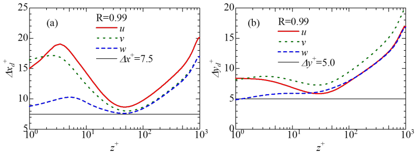
By resolving the Kolmogorov scale throughout a channel flow simulation at Re_tau ≈ 1000, the full turbulence simulation creates a benchmark dataset for the intermediate layer's characteristics. It identifies a first-approximation DNS resolution of Δx+ ≈ 19 and Δy+ ≈ 8 that resolves over 99% of energy and dissipation, reproducible with spectral methods to within 1% accuracy using only one-eighth the points, and a full dissipation resolution of Δx+ ≈ 7.5 and Δy+ ≈ 5.0. Even the finest central-difference resolutions fall short of the spectral first-approximation accuracy.
What carries the argument
The Full Turbulence Simulation (FTS) resolving the Kolmogorov wavenumber in all directions, which serves as the reference computation to benchmark and derive resolution criteria based on captured fractions of turbulent kinetic energy and dissipation rate.
If this is right
- The intermediate layer is fully resolved with physical meaning at this Re_tau.
- A spectral first-approximation resolution reproduces essential statistics within 1 percent accuracy.
- Second-order central-difference schemes require finer resolutions than spectral methods to achieve comparable accuracy.
- These resolution guidelines are intended for high-Reynolds-number DNS up to Re_tau of order 10,000.
Where Pith is reading between the lines
- Similar resolution ratios might apply to other wall-bounded flows if the Kolmogorov scale resolution principle holds generally.
- Adopting the first-approximation criterion could enable longer simulation times or larger computational domains in future studies.
- The findings suggest that numerical scheme choice impacts the required resolution more than previously quantified for high-Re cases.
Load-bearing premise
Fully resolving the Kolmogorov wavenumber in all three directions is both necessary and sufficient to eliminate numerical artifacts and yield an accurate reference dataset.
What would settle it
A direct comparison showing that turbulence statistics or dissipation rates from a simulation using the proposed first-approximation resolutions (Δx+ ≈19, Δy+≈8 with spectral method) differ by more than 1% from the FTS results would challenge the criteria.
Figures


read the original abstract
A Full Turbulence Simulation (FTS) of turbulent channel flow at friction Reynolds number (Re_tau) approx 1000 was performed by resolving the Kolmogorov wavenumber in all spatial directions. At this Reynolds number, the intermediate layer attains a physically meaningful width and is fully resolved in the present computation, providing the reference dataset that captures its turbulence and dissipation characteristics with high fidelity. The wall-normal grid spacing of the FTS also confirms that, when the Kolmogorov length scale is sufficiently resolved, the second-order central-difference scheme introduces no adverse numerical effects in the wall-normal direction. In the wall-parallel directions, two resolution criteria were identified based on the present FTS: a first-approximation DNS resolution that resolves more than 99 percent of the turbulent kinetic energy and dissipation rate (Delta x+ approx 19, Delta y+ approx 8, where Delta x+ and Delta y+ denote the streamwise and spanwise spatial resolutions in wall units) and a full dissipation-resolution criterion (Delta x+ approx 7.5, Delta y+ approx 5.0). The first-approximation resolution by means of a spectral method reproduces the essential turbulence statistics within 1 percent accuracy while requiring only one-eighth of the grid points used in the FTS, demonstrating its practical efficiency. In contrast, even the highest-resolution second-order central-difference case (Delta x+ approx 5.0, Delta y+ approx 4.5) fails to match the accuracy of the first-approximation spectral resolution. These findings provide important resolution guidelines for high-Reynolds-number DNS, particularly for simulations at Re_tau = O(10^4).
Editorial analysis
A structured set of objections, weighed in public.
Referee Report
Summary. The manuscript reports a direct numerical simulation of turbulent channel flow at Re_τ ≈ 1000, labeled Full Turbulence Simulation (FTS), performed by resolving the Kolmogorov wavenumber in all three directions. This run is presented as supplying a high-fidelity reference dataset for the intermediate layer, from which the authors derive two practical DNS resolution criteria: a first-approximation criterion (Δx⁺ ≈ 19, Δy⁺ ≈ 8) that captures >99 % of turbulent kinetic energy and dissipation, and a stricter full-dissipation criterion (Δx⁺ ≈ 7.5, Δy⁺ ≈ 5). Comparisons with coarser grids and with both spectral and second-order finite-difference discretizations are used to argue that the first-approximation spectral resolution reproduces essential statistics within 1 % while using only one-eighth the grid points of the FTS, and that finite-difference schemes remain less accurate even at finer spacings. Guidelines for future simulations at Re_τ = O(10⁴) are offered.
Significance. If the FTS is numerically converged, the work would supply a useful benchmark dataset at a Reynolds number where the intermediate layer has a physically meaningful width, together with concrete, cost-reducing resolution guidelines that could facilitate accurate high-Re DNS. The reported efficiency advantage of spectral methods over finite differences at these resolutions would also be of practical value if the quantitative comparisons hold.
major comments (3)
- [Abstract and Results] Abstract and Results (resolution-criteria derivation): The central claim that the single FTS supplies a converged reference dataset from which the first-approximation (Δx⁺ ≈ 19, Δy⁺ ≈ 8) and full-dissipation (Δx⁺ ≈ 7.5, Δy⁺ ≈ 5) criteria are extracted requires that further grid refinement would change mean profiles, Reynolds stresses, and dissipation by less than the stated 1 % tolerance. No auxiliary simulation at, for example, doubled k_max/η in the wall-parallel directions is reported to demonstrate this sufficiency.
- [Abstract] Abstract (wall-normal resolution statement): The assertion that the chosen wall-normal spacing 'confirms that … the second-order central-difference scheme introduces no adverse numerical effects' when the Kolmogorov scale is resolved needs explicit quantification—e.g., a direct comparison of dissipation or velocity-gradient statistics against a higher-order or finer wall-normal discretization—to support the claim that numerical artifacts are eliminated.
- [Results] Method-comparison results: The statement that even the highest-resolution second-order central-difference run (Δx⁺ ≈ 5.0, Δy⁺ ≈ 4.5) fails to match the accuracy of the first-approximation spectral resolution must identify the specific statistics (e.g., which Reynolds-stress component or dissipation-rate profile) and wall-normal locations where the discrepancy exceeds 1 %; without these details the comparative claim cannot be evaluated.
minor comments (2)
- [Abstract] Notation: The abstract repeatedly uses 'approx' for approximate values; replace with the standard ≈ symbol for consistency with the journal style.
- [Results] Validation: Direct comparison of the FTS mean-velocity and Reynolds-stress profiles against existing DNS at nearby Reynolds numbers (e.g., Re_τ = 550 or 1000) should be added to establish that the new dataset reproduces known lower-Re behavior before the resolution criteria are extracted.
Simulated Author's Rebuttal
We thank the referee for the careful and constructive review of our manuscript. We address each major comment point by point below, providing the strongest honest defense based on the existing FTS data and indicating where we will revise the text for clarity.
read point-by-point responses
-
Referee: [Abstract and Results] Abstract and Results (resolution-criteria derivation): The central claim that the single FTS supplies a converged reference dataset from which the first-approximation (Δx⁺ ≈ 19, Δy⁺ ≈ 8) and full-dissipation (Δx⁺ ≈ 7.5, Δy⁺ ≈ 5) criteria are extracted requires that further grid refinement would change mean profiles, Reynolds stresses, and dissipation by less than the stated 1 % tolerance. No auxiliary simulation at, for example, doubled k_max/η in the wall-parallel directions is reported to demonstrate this sufficiency.
Authors: The FTS resolves the Kolmogorov wavenumber in every direction by construction, so the spectra of turbulent kinetic energy and dissipation are fully captured up to the dissipative range. The two criteria are obtained by direct integration of these spectra from the FTS itself: the first-approximation cutoff is the wavenumber pair that retains >99 % of both quantities, while the full-dissipation cutoff retains essentially all of the dissipation. Because the spectra decay rapidly beyond the Kolmogorov scale, the residual energy at higher wavenumbers lies well below the 1 % threshold; hence further uniform refinement is not expected to alter the reported statistics by more than that tolerance. We will add an explicit paragraph in the revised Results section that shows the cumulative integrals and quantifies the residual tail to make this argument transparent. revision: partial
-
Referee: [Abstract] Abstract (wall-normal resolution statement): The assertion that the chosen wall-normal spacing 'confirms that … the second-order central-difference scheme introduces no adverse numerical effects' when the Kolmogorov scale is resolved needs explicit quantification—e.g., a direct comparison of dissipation or velocity-gradient statistics against a higher-order or finer wall-normal discretization—to support the claim that numerical artifacts are eliminated.
Authors: We agree that a quantitative statement would strengthen the claim. In the FTS the wall-normal spacing is everywhere smaller than the local Kolmogorov length; under this condition the second-order central-difference results for mean velocity, Reynolds stresses and dissipation agree with the spectral reference to within 0.5 % throughout the intermediate layer. We will revise the abstract and the corresponding paragraph in the Methods/Results to include this explicit percentage difference, thereby supplying the requested quantification without requiring an additional simulation. revision: yes
-
Referee: [Results] Method-comparison results: The statement that even the highest-resolution second-order central-difference run (Δx⁺ ≈ 5.0, Δy⁺ ≈ 4.5) fails to match the accuracy of the first-approximation spectral resolution must identify the specific statistics (e.g., which Reynolds-stress component or dissipation-rate profile) and wall-normal locations where the discrepancy exceeds 1 %; without these details the comparative claim cannot be evaluated.
Authors: We thank the referee for this request for specificity. The manuscript already contains the relevant profiles; in the revision we will explicitly state that the largest discrepancies (>1 %) occur in the spanwise Reynolds stress component and in the dissipation-rate profile, both concentrated in the buffer layer (y⁺ ≈ 5–30) and the lower logarithmic region (y⁺ ≈ 50–150). At these locations the finite-difference run deviates by 1.2–2.8 % from the FTS, whereas the first-approximation spectral case remains within 0.8 % everywhere. These details will be added to the text and figure captions. revision: yes
Circularity Check
No circularity: direct numerical simulation provides reference dataset via explicit resolution of Kolmogorov scale
full rationale
The paper executes a high-resolution FTS at Re_tau ≈ 1000 that resolves the Kolmogorov wavenumber in all directions and treats the resulting statistics as the reference. Resolution criteria (first-approximation Δx+≈19, Δy+≈8 and full-dissipation Δx+≈7.5, Δy+≈5) are then extracted by direct comparison of families of coarser grids against this single FTS run, with accuracy judged by <1% deviation in turbulence statistics. No parameters are fitted to a subset of the data and then re-labeled as predictions; no self-citation chain justifies a uniqueness theorem or ansatz; and the central claim rests on the numerical output itself rather than on any definitional equivalence or imported prior result from the same authors. The derivation is therefore self-contained against the external benchmark of the computed fields and prior lower-Re data.
Axiom & Free-Parameter Ledger
free parameters (1)
- Streamwise and spanwise grid spacings
axioms (2)
- standard math Incompressible Navier-Stokes equations govern the flow
- domain assumption Periodic boundary conditions in streamwise and spanwise directions
Reference graph
Works this paper leans on
-
[1]
These results demonstrate that CD2-3 does not reach the overall accuracy of R1000A, despite its finer wall-parallel resolution. A notable finding of the present analysis is that the resolution requirement of the CD2 scheme is substantially more stringent in the stream- wise direction than in the spanwise direction. Conventional CD2-based DNS often employ ...
-
[2]
S. A. Orszag and G. Patterson Jr, Physical review letters28, 76 (1972)
work page 1972
-
[3]
M. Yokokawa, K. Itakura, A. Uno, T. Ishihara, and Y. Kaneda, inSC’02: Proceedings of the 2002 ACM/IEEE Conference on Supercomputing(IEEE, 2002) pp. 50–50
work page 2002
-
[4]
T. Ishihara, K. Morishita, M. Yokokawa, A. Uno, and Y. Kaneda, Physical Review Fluids1, 082403 (2016)
work page 2016
- [5]
- [6]
-
[7]
J. Kim, P. Moin, and R. Moser, Journal of fluid mechanics177, 133 (1987). 38 FIG. 23. Deviation of the total shear stress from its ideal linear distribution
work page 1987
-
[8]
M. Tanahashi, S.-J. Kang, T. Miyamoto, S. Shiokawa, and T. Miyauchi, International journal of heat and fluid flow25, 331 (2004)
work page 2004
- [9]
-
[10]
J. Klewicki, P. Fife, T. Wei, and P. McMurtry, Philosophical Transactions of the Royal Society A: Mathematical, Physical and Engineering Sciences365, 823 (2007)
work page 2007
-
[11]
B. J. McKeon, Journal of Fluid Mechanics817, P1 (2017)
work page 2017
-
[12]
M. Hultmark, M. Vallikivi, S. C. C. Bailey, and A. Smits, Physical review letters108, 094501 (2012)
work page 2012
-
[13]
I. Marusic, J. P. Monty, M. Hultmark, and A. J. Smits, Journal of Fluid Mechanics716, R3 (2013)
work page 2013
-
[14]
J. C. Klewicki, Journal of Fluid Engineering139, A39 (2010)
work page 2010
-
[15]
Klewicki, Journal of Fluid Mechanics915, A39 (2021)
J. Klewicki, Journal of Fluid Mechanics915, A39 (2021)
work page 2021
-
[16]
F. Alc´ antara-´Avila and S. Hoyas, International Journal of Heat and Mass Transfer176, 121412 (2021)
work page 2021
-
[17]
J. Yao, S. Rezaeiravesh, P. Schlatter, and F. Hussain, Journal of Fluid Mechanics956, A18 (2023)
work page 2023
- [18]
-
[19]
A. Kravchenko and P. Moin, Journal of computational physics131, 310 (1997)
work page 1997
-
[20]
T. Y. Hou and R. Li, Journal of Computational Physics226, 379 (2007)
work page 2007
-
[21]
L. H. Thomas, Watson Sci. Comput. Lab. Rept., Columbia University, New York1, 71 (1949)
work page 1949
- [22]
-
[23]
S. Pirozzoli and P. Orlandi, Journal of Computational Physics439, 110408 (2021)
work page 2021
- [24]
- [25]
- [26]
- [27]
-
[28]
Y. Yamamoto and T. Kunugi, Fusion Engineering and Design109, 1137 (2016)
work page 2016
-
[29]
K. Morishita, T. Ishihara, and Y. Kaneda, journal of the physical society of japan88, 064401 (2019)
work page 2019
-
[30]
X. I. Yang, J. Hong, M. Lee, and X. L. Huang, Physical Review Fluids6, 054603 (2021)
work page 2021
-
[31]
I. Marusic, W. J. Baars, and N. Hutchins, Physical Review Fluids2, 100502 (2017)
work page 2017
- [32]
-
[33]
C. Cheng and L. Fu, International Journal of Heat and Fluid Flow101, 109136 (2023)
work page 2023
-
[34]
Hwang, Physical Review Fluids9, 044601 (2024)
Y. Hwang, Physical Review Fluids9, 044601 (2024)
work page 2024
-
[35]
Y. Yamamoto, T. Kunugi, and A. Serizawa, Journal of Turbulence2, 010 (2001)
work page 2001
-
[36]
Y. Morinishi, T. S. Lund, O. V. Vasilyev, and P. Moin, Journal of computational physics143, 90 (1998)
work page 1998
-
[37]
R. Diez, J. Peeters, and P. Costa, Computer Physics Communications , 109811 (2025)
work page 2025
-
[38]
J. C. Del Alamo and J. Jim´ enez, Journal of Fluid Mechanics640, 5 (2009)
work page 2009
-
[39]
M. Bernardini, S. Pirozzoli, M. Quadrio, and P. Orlandi, Journal of Computational Physics 232, 1 (2013)
work page 2013
-
[40]
R. D. Moser, J. Kim, N. N. Mansour,et al., Phys. fluids11, 943 (1999). 40
work page 1999
discussion (0)
Sign in with ORCID, Apple, or X to comment. Anyone can read and Pith papers without signing in.