Geometric control theory of vertical rolling disc using symmetries

Ales Navrat; Jaroslav Hrdina; Lenka Zalabova

REVIEW 2 major objections 5 minor 34 references

Geometric control theory of vertical rolling disc using symmetries

T0 review · 2 major / 5 minor · reviewed 2026-08-14 · deepseek-v4-flash

Challenge this review Re-run · record.json Download PDF Read on arXiv ↗ Review JSON

Pith's one-line read The paper proves that each generic geodesic in the nilpotent rolling-disc model first stops being optimal exactly where a rotational symmetry fixes it, and gives the location explicitly.

desk verdict A sound, honest methods paper that re-derives known Heisenberg results for the rolling disc; the useful contribution is the reproducible Maple computation, not a new theorem. read the letter →

arxiv 1908.03352 v1 pith:4IJANZ5V submitted 2019-08-09 math.DG

Jaroslav Hrdina , Ales Navrat , Lenka Zalabova This is my paper · ORCID

classification math.DG MSC 53C1770Q0522E6037J60

keywords verticalrollingdiscnilpotentapproximationHeisenberggroupsub-RiemanniangeometrycutpointisotropysymmetryLagrangiancontactstructuremaximumprinciple

verification ladder T0 review T1 audit T2 compute T3 formal

The pith

A machine-rendered reading of the paper's core claim, the machinery that carries it, and where it could break.

The reading

The paper studies optimal movement of a vertical rolling disc as a sub-Riemannian control problem and replaces the intractable extremal equations by a homogeneous nilpotent approximation modelled on the three-dimensional Heisenberg group. In that model every generic length-minimizing curve can be written explicitly, and the paper proves that a one-dimensional rotational symmetry fixes the exact point where each such curve first ceases to be optimal: the first cut point. The argument identifies this point directly from the symmetry's fixed-point set, without solving a separate optimality problem. The paper further proves that the Lagrangian contact structure, which keeps angular and plane velocities distinguished, has symmetry algebra $\mathfrak{sl}(3,\mathbb{R})$, and that no positive-definite sub-Riemannian metric is invariant under that full symmetry group. Explicit cut points matter because they are what make sub-Riemannian distance and motion planning tractable on the model that approximates the rolling disc.

What carries the argument

The load-bearing object is the isotropy symmetry $t_0$, a vector field whose flow rotates the horizontal distribution around the origin and whose fixed-point set is the line $S=\{(0,y,0)\}$. Applying $t_0$ to a local minimizer from (30) maps it to other local minimizers from the origin with the same parametrization and the same endpoint at time $2\pi/C_1$; a symmetry with this property gives a direct certificate that the curve stops being optimal at the meeting point. Around this, the machinery is the left-invariant Hamiltonian description of the Heisenberg-group control problem, which splits extremals into the vertical system (27) and horizontal system (28), and the translation symmetries $t_1,t_2,t_3$ that move solutions between different initial conditions. For the Lagrangian contact structure, the algebraic prolongation of the grading $g_{-2}\oplus g_{-1}$ yields the full symmetry algebra $\mathfrak{sl}(3,\mathbb{R})$, and the action of its degree-zero part on $g_{-1}$ rules out any invariant positive-definite metric.

What would settle it

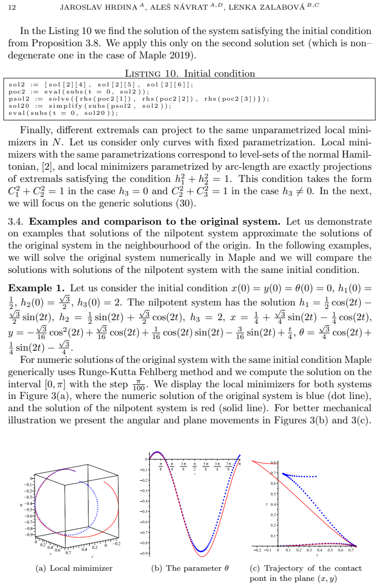
For the nilpotent system with $C_1=2$ and $C_2^2+C_3^2=1$ (as in Example 1), the proposition predicts the first cut point $(0,\pi/4,0)$ at time $\pi$; solve the original rolling-disc extremal system numerically with the same initial covector and test whether any admissible curve shorter than the extremal connects the origin to that point before time $\pi$. If such a shorter curve exists, or if the first intersection of the true extremal with $x=\theta=0$ occurs at a value of $y$ different from the nilpotent prediction, the approximation does not control the original cut locus.

Watch

Extended reading notes

Core claim

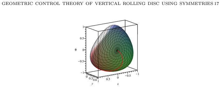
The central result is Proposition 4.4. In the nilpotent approximation with coordinates $(\theta,x,y)$, every local minimizer from (30) with $h_3=C_1\neq 0$ and $C_2C_3\neq 0$ intersects the fixed-point set $S=\{(0,y,0)\}$ of the isotropy symmetry $t_0 = \theta\,\partial_x + \frac{\theta^2-x^2}{2}\,\partial_y - x\,\partial_\theta$ at the point $(0,\pi(C_2^2+C_3^2)/C_1^2,0)$ at time $2\pi/C_1$, and this is the first such intersection. Since two equal-length extremals meeting at the same point and time cannot be optimal past the meeting point, this intersection is the first cut point along the minimizer; for arc-length parametrized curves, where $C_2^2+C_3^2=1$, it simplifies to $(0,\pi/C_1^2,0)$. The isotropy flow simultaneously produces a one-parameter family of equal-length minimizers from the origin to that point. The paper also establishes, by algebraic prolongation of the contact grading, that the symmetry algebra of the Lagrangian contact structure is $\mathfrak{sl}(3,\mathbb{R})$, and that no positive-definite sub-Riemannian metric is invariant under that algebra.

Load-bearing premise

The first-cut-point theorem is proved in the nilpotent approximation; the paper assumes, without a rigorous error estimate, that this approximation faithfully represents where geodesics of the original rolling disc stop being optimal.

Editorial extensions

If this is right

For the nilpotent approximation, every generic arc-length minimizer has its first cut point on the line $S$ at $(0,\pi/C_1^2,0)$, so the first cut locus is explicitly parametrized by $C_1$.
Because the isotropy flow generates a one-parameter family of equal-length minimizers between the origin and each cut point, the cut locus near the origin is the rotational image of a single generic minimizer.
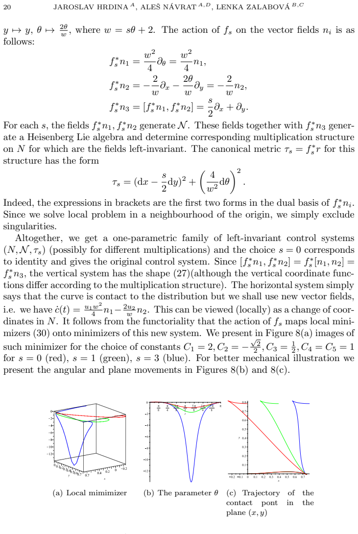
The translation symmetries mean a solution starting anywhere in a neighbourhood can be obtained from the origin solution by the group law with the same vertical covector, so the explicit formulas (30) solve every nearby optimal-control problem, not only those starting at the origin.
The symmetry algebra $\mathfrak{sl}(3,\mathbb{R})$ has maximal possible dimension for a three-dimensional Lagrangian contact structure, so the nilpotent model is flat in the parabolic-geometry sense; all metrics that preserve the angular/plane velocity splitting but vary the unit ratio are related by these symmetries.
Since no positive-definite metric is invariant under $\mathfrak{sl}(3,\mathbb{R})$, any choice of units for angular versus plane velocity breaks the full symmetry, leaving exactly the three translations as the metric-preserving symmetry group.

Reading between the lines

Editorial extensions of the paper, not claims the author makes directly.

A natural but unproved conjecture is that the first cut time of the original rolling disc converges to $2\pi/C_1$ as the endpoint approaches the origin; the paper's two numerical examples are consistent with this, but Section 3.4 gives no error estimate.
The same symmetry argument should apply to any control system with the same three-dimensional solvable controllability algebra, such as the reduced kinematic-car system (11), giving the same first cut-point formula after a coordinate change.
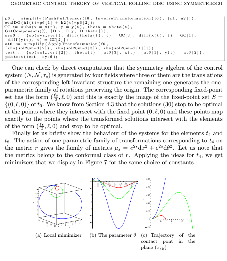
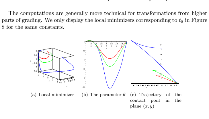
The $\mathfrak{sl}(3,\mathbb{R})$ symmetry suggests a motion-planning shortcut: instead of re-solving the extremal equations for each choice of velocity-unit ratio, one can pull known Heisenberg minimizers back through the symmetry flow and compare their cost under the family of metrics $\tau_s$.
A sharper structural test would be to reduce the Heisenberg geodesic flow by the isotropy symmetry $t_0$; the fixed-point set $S$ should then appear as a caustic or conjugate locus in the reduced space, giving a symplectic explanation of the first cut time.

Share X Bluesky LinkedIn Reddit HN

Signed reviews

No signed human review yet.

Editorial analysis

A structured set of objections, weighed in public.

Desk editor's note, referee report, and a circularity audit.

Desk Editor's Note

read the letter

Dear X,

Read the Hrdina–Navrat–Zalabova paper. Quick take: it's a clean, honest methods paper about the Heisenberg nilpotent approximation of the vertical rolling disc, not a new-theorem paper. Most of the mathematical content is a re-derivation of known results — the nilpotent approximation, the explicit geodesics, the isotropy symmetry and the cut point are all in [2] and [26], and the sl(3,R) symmetry algebra of the Lagrangian contact structure is standard parabolic geometry. The paper says so. Its value is in the explicit, self-contained derivations and the Maple/DifferentialGeometry code, which is real reproducible evidence.

What it does well: PMP setup is correct, vertical and horizontal systems check out, solutions (29)-(30) are explicit and satisfy the equations, the symmetry computation via Tanaka prolongation in Appendix A is detailed, and Lemma 5.4 is neatly proven. The numerical comparison in Section 3.4 is honest — two examples, no error estimates, but presented as demonstration. The attribution of the cut point to [2,26] is exactly right.

Soft spots: Two. First, the cut-point discussion in Section 4 is only about the nilpotent model, and Prop 4.4 alone establishes at most an upper bound on the cut time: the orbit of the isotropy symmetry gives a distinct local minimizer with the same endpoint at t=2π/C1, which means optimality ceases at or before that time; equality requires the known conjugate-locus results, which the paper cites but could be more explicit about when presenting Prop 4.4 as a 'recovery' of the cut point. Second, the transfer from the nilpotent model to the actual rolling disc is informal. The paper never proves that the cut locus of the approximation controls the cut locus of the disc, and the two numerical comparisons in Section 3.4 don't amount to an estimate. The paper is careful not to overclaim — Remark 4.2 notes the original structure lacks the isotropy symmetry — but the title and framing might lead a reader to think the cut-point result applies to the disc. One sentence of scope limitation would fix it.

Who is this for: someone wanting a worked, executable example of symmetry methods in sub-Riemannian control, or checking Maple implementations. It deserves peer review — it's sound, self-contained, and reproducible — but expect the referee to ask for a clearer statement of what is genuinely new and a tighter discussion of the nilpotent approximation's limits.

FWIW, I'd send it out rather than desk-reject.

Referee Report

2 major / 5 minor

Summary. The paper studies the vertical rolling disc as a nonholonomic control system, derives the Pontryagin extremal equations for the original system and for its homogeneous nilpotent approximation, and then focuses on the Heisenberg nilpotent model. It gives explicit solutions of the extremal equations (Propositions 3.7 and 3.8), computes the full infinitesimal symmetry algebra of the sub-Riemannian structure (Proposition 4.1), and uses the isotropy symmetry t0 to construct a one-parameter family of local minimizers with a common endpoint in the fixed-point set S (Proposition 4.4 and Corollary 4.5). The paper then studies the Lagrangian contact structure of the nilpotent model, proves that its symmetry algebra is sl(3,R) (Proposition 5.2), and shows that no positive definite sub-Riemannian metric is invariant under this full symmetry algebra (Lemma 5.4). The text is accompanied by extensive Maple/DifferentialGeometry code and several numerical comparisons with the original rolling-disc system.

Significance. The paper is a careful, self-contained computation in the geometric control of the Heisenberg nilpotent model associated with the vertical rolling disc. The explicit solutions in Proposition 3.8, the symmetry classification in Propositions 4.1 and 5.2, and the non-existence result in Lemma 5.4 are cleanly stated and are supported by reproducible CAS code and direct verification of the differential equations. The symmetry-based construction in Section 4.3 gives a transparent geometric explanation of the known Heisenberg conjugate/cut-locus results, and the discussion of the metric class attached to the Lagrangian contact structure is a useful contribution. The main limitation is that the cut-point and symmetry results are proven for the nilpotent approximation only; the connection to the original rolling disc is made through numerical examples and informal statements, not through quantitative estimates.

major comments (2)

[Section 4.3, Proposition 4.4] The proof establishes that, for each generic extremal (30), the isotropy flow produces a one-parameter family of distinct local minimizers with the same endpoint at time t=2*pi/C1, which shows that the geodesic cannot be optimal after that time. This is an upper bound on the cut time. The phrase "and it is the first point with this property" refers to the first intersection with the fixed-point set S, not the first cut point. If the authors intend Proposition 4.4 and Corollary 4.5 to assert equality with the cut point, an additional argument (for example, a conjugate-point or distance comparison) is required; as written, the equality is only supported by the citations [2,26] mentioned after Corollary 4.5. Please make the exact logical status of the cut-point claim explicit.
[Sections 3.4 and 4.3 (scope)] The numerical comparison in Section 3.4 is purely visual and contains no error estimate, and Remark 4.2 explicitly states that the original rolling-disc structure has no isotropy symmetry analogous to t0. Consequently, the cut-point and symmetry results in Section 4 are established only for the nilpotent Heisenberg model, not for the vertical rolling disc itself. The title, the abstract, and the sentence in Section 3 saying that the nilpotent approximation "still describes the system appropriately" should be qualified to reflect this, or a quantitative transfer statement must be supplied. As written, a reader could reasonably infer a cut-locus statement for the original system that is not proved.

minor comments (5)

[Proposition 4.4] The condition C2*C3 different from 0 is stronger than needed: the first-intersection computation with S also works when exactly one of C2, C3 vanishes, and the genuinely degenerate case to exclude is C2=C3=0. In addition, the time 2*pi/C1 should be written as 2*pi/|C1|, or the authors should state explicitly that C1>0 is assumed.
[Section 5.4] The displayed formula for tau_s contains (dx - s/2 dy)^2, but the flow is x maps to x + s y/2, so the pullback of r=dx^2+d theta^2 gives (dx + s/2 dy)^2. Please check this sign and also clarify the convention used for f_s^* on vector fields, since the factors w^2/4 and 4/w^2 appear inverted relative to the usual pushforward convention.
[Appendix A] The displayed formula for Ye7 is missing the final basis vector: it should read Ye7 = 2x^2*dx + 2xy*dy + (2y - x*theta)*d_theta.
[Table 2] The bracket table appears to use the convention that the entry in row i and column j represents [e_j, e_i] rather than the more common [e_i, e_j]. Please state the convention explicitly or transpose the table to avoid confusion.
[Section 1.1] The text contains the typo "Im other words"; it should read "In other words".

Circularity Check

0 steps flagged · score 0.0 of 10

No significant circularity; central derivations are self-contained, and external references are not load-bearing.

full rationale

The paper's central chain is self-contained: PMP yields the extremal systems (17,18) and (27,28); explicit integration gives the solutions (29) and (30); the symmetry t0 is obtained by explicitly solving PDEs in Proposition 4.1; and Proposition 4.4 then solves x=theta=0 for the explicit curve (30), obtaining t=2*pi/C1 and evaluating y. None of these steps uses a fitted parameter or a self-citation as an input. The only citations used in the derivation are standard external references for PMP, nilpotent approximation, and the known Heisenberg conjugate-locus result ([2,26]); the authors' own works [18]-[21] appear only in peripheral contexts and are not load-bearing for Proposition 4.4, Proposition 5.2, or Lemma 5.4. The numerical comparison in Section 3.4 and Remark 4.2 explicitly limit the symmetry/cut analysis to the nilpotent model, which is a transfer limitation rather than a circular reduction. Thus no claimed step reduces by construction to its own input.

Assumptions & free parameters 1 free parameters · 4 assumptions · 0 invented entities

The paper introduces no new physical or abstract entities. The vector fields t0...t8 are standard generators of symmetry algebras, and the constants C1,C2,C3 are integration constants. The assumptions are the standard modeling assumptions for the rolling disc and the standard background theorems.

free parameters (1)

C1, C2, C3 in the explicit solutions (29), (30) = arbitrary integration constants
These constants parametrize the solutions of the vertical system and are not fit to data. They play the role of covectors in the PMP, not fitted parameters.

assumptions (4)

domain assumption The vertical rolling disc without slipping is modeled by the nonholonomic Pfaff system dx - cos(theta)dphi = 0, dy - sin(theta)dphi = 0, and after eliminating phi by dy cos(theta) - dx sin(theta) = 0.
This is the physical modeling assumption that the disc has unit radius and rolls without slipping. It enters in Section 1.1.
domain assumption The configuration space of the disc can locally be viewed as a connected, simply connected Lie group K whose left-invariant fields are X1, X2, X12.
This assumption in Section 2.1 allows the use of left-invariant Hamiltonian techniques and the PMP on a Lie group. It is valid locally, though the global configuration space S^1 x R^2 is not the simply connected group SE(2).
ad hoc to paper The nilpotent approximation accurately describes the original system near the origin for the purpose of computing local minimizers and cut loci.
This is used implicitly in Sections 3.4 and 4.3. The paper only gives numerical examples, no rigorous error bound.
standard math Standard theorems of sub-Riemannian geometry, including Chow-Rashevskii controllability, Pontryagin's maximum principle, and the Tanaka prolongation procedure.
These are external results cited in [2], [22], [32], [34] and used throughout the paper without proof.

how reviews work

0 comments

Cite this review

Pith. "Pith review of Geometric control theory of vertical rolling disc using symmetries." pith.science (2026). https://pith.science/paper/4IJANZ5V

@misc{pith2026190803352,
  author       = {Pith},
  title        = {Pith review of: Geometric control theory of vertical rolling disc using symmetries},
  year         = {2026},
  howpublished = {\url{https://pith.science/paper/4IJANZ5V}},
  note         = {Machine review of arXiv:1908.03352}
}

read the original abstract

We use the methods of geometric control theory to study extremal trajectories of vertical rolling disk. We focus on the role of symmetries of the underlying geometric structures. We demonstrate the computations in the CAS Maple package DifferentialGeometry.

Figures

Figures reproduced from arXiv: 1908.03352 by the authors.

**Figure 1.** Vertical rolling disc radius of the disc equals to 1. We assume that the rolling of the disc is without slipping nor sliding. Im other words, we suppose that the direct plane velocity of the disc is proportional to angular velocity of the circular motion. In coordinates, the nonholonomic constraints are x˙ = cos θϕ,˙ y˙ = sin θϕ.˙ (1) We can reformulate equations (1) in the formalism of differential forms as a Pfaff… view at source ↗

**Figure 2.** Kinematic car The Pfaffian constraints on the admissible movements of the car are sin(θ + ϕ) ˙x − cos(θ + ϕ) ˙y − ` cos ϕ ˙θ = 0, sin θx˙ − cos θy˙ = 0. (10) The corresponding control system with the inputs chosen as the plane velocity u1 = ˙ϕ and the angular velocity u2 has the form ˙q = u1Z1 + u2Z2 for Z1 = ∂ϕ, Z2 = cos θ∂x + sin θ∂y + tan ϕ ` ∂θ. We would like to discuss the relation of this system with the syste… view at source ↗

**Figure 3.** Comparing of the analytic solution of approximation and the numeric solution of the original system: Example 1 Example 2. Let us now consider the initial condition x(0) = y(0) = θ(0) = 0, h1(0) = 1 2 , h2(0) = √ 3 2 , h3(0) = 20. The nilpotent system has the solution [PITH_FULL_IMAGE:figures/full_fig_p012_3.png] view at source ↗

Figures from the paper (5 more)

**Figure 4.** Figure 4: Comparing of the analytic solution of approximation and the numeric solution of the original system: Example 2 Let us note that our choice is such that in both cases, we display one period of the graphs and we have evenly distributed 100 points in the interval. 4. Symm…

**Figure 5.** Figure 5: One parametric family of local minimizers rolling disc and the generators n1, n2 naturally correspond to the angular velocity and plane velocity. Thus the choice of n1 and n2 gives the choice of units of the two velocities which then impacts the metric and local optima…

**Figure 6.** Figure 6: Action of one–parametric family for t6 In Listing 17, we check by direct computation that transformed curves are solutions of the transformed system. Listing 17. Action on solutions pso l2mod := s o l v e ({ r h s ( poc2 [ 1 ] ) , r h s ( poc2 [ 2 ] ) , r h s ( poc2 […

**Figure 7.** Figure 7: Action of one–parametric family for t4 The computations are generally more technical for transformations from higher parts of grading. We only display the local minimizers corresponding to t8 in [PITH_FULL_IMAGE:figures/full_fig_p021_7.png]

**Figure 8.** Figure 8: Action of one–parametric family for t8 [PITH_FULL_IMAGE:figures/full_fig_p021_8.png]

Discussion (0). Continue with ORCID to comment.

Reference graph

Works this paper leans on

34 extracted references · 31 canonical work pages

[2]

A. A. Agrachev, D. Barilari and U. Boscain , A Comprehensive Introduction to sub– Riemannian geometry Cambridge Studies in Advanced Mathematics, Cambridge University Press, 2019

work page 2019
[26]

Monroy-Prez and A

F. Monroy-Prez and A. Anzaldo-Meneses , Optimal Control on the Heisen- berg Group Journal of Dynamical and Control Systems (1999) 5: 473. https://doi.org/10.1023/A:1021787121457

work page doi:10.1023/a:1021787121457 1999
[1]

A. A. Agrachev and Y. L. Sachkov , Control theory from the geometric viewpoint , Ency- clopaedia of Mathematical Sciences, Control Theory and Optimization, Springer (2006)

work page 2006
[3]

Constant Curvature Models in Sub-Riemannian Geometry

D. Alekseevsky, A. Medvedev and J. Slovak , Constant Curvature Models in Sub- Riemannian Geometry , arXiv:1712.10278 [math.DG], 2018

work page Pith review arXiv 2018
[4]

A. A. Agrachev and A. V. Sarychev , Filtrations of a lie algebra of vector ﬁelds and the nilpotent approximation of controllable systems Dokl. Akad. Nauk SSSR, 295(4):104–108, 1987

work page 1987
[5]

I. M. Anderson and C. G. Torre , New symbolic tools for diﬀerential geometry, gravitation, and ﬁeld theory. J. Math. Phys. , 53(013511):1–12, 2012

work page 2012
[6]

Bellaiche, The tangent space in sub–Riemannian geometry , Sub-Riemannian Geometry, Birkh¨ auser Basel, pp

A. Bellaiche, The tangent space in sub–Riemannian geometry , Sub-Riemannian Geometry, Birkh¨ auser Basel, pp. 1–78 (1996)

work page 1996
[7]

Beschastnyi and A

I. Beschastnyi and A. Medvedev , Left-Invariant Sub-Riemannian Engel Structures: Ab- normal Geodesics and Integrability , SIAM J. Control Optim., 56(5), pp. 3524-3537 (2018)

work page 2018

Show all 34 references

[8]

ˇCap and J

A. ˇCap and J. Slov´ak, Parabolic geometries I, Background and general theory, , volume 154. AMS Publishing House, 2009

2009
[9]

Bloch, Nonholonomic Mechanics and Control , Springer 2015, pp

A.M. Bloch, Nonholonomic Mechanics and Control , Springer 2015, pp. 565

2015
[10]

Calin, D

O. Calin, D. Ch. Chang and P. Greiner , Geometric Analysis on the Heisenberg Group and Its Generalizations , AMS/IP Studies in advanced mathematics, American Mathematical Society 2008

2008
[11]

Calin and D

O. Calin and D. Chang, Sub-Riemannian Geometry: General Theory and Examples (Ency- clopedia of Mathematics and its Applications). Cambridge: Cambridge University Press.(2009) 26 JAROSLAV HRDINA A, ALEˇS N ´AVRAT A,D, LENKA ZALABOV ´A B,C

2009
[12]

K. L. Doty, C. Melchiorri and C. Bonivento , A Theory of Generalized Inverses Applied to Robotics, Internatinal Journal of Robotics Research, Sage Publications vol. 12, Issue. 1, pp. 1-19 (1993)

1993
[13]

Dubins, On Curves of Minimal Length with a Constraint on Average Curvature, and with Prescribed Initial and Terminal Positions and Tangents , American Journal of Mathe- matics

L.E. Dubins, On Curves of Minimal Length with a Constraint on Average Curvature, and with Prescribed Initial and Terminal Positions and Tangents , American Journal of Mathe- matics. 79 (3): 497–516
[14]

Eastwood and P

M. Eastwood and P. Nurowski , Aerodynamics of ﬂying saucers, arXiv:1810.04855 (2018)

2018 arXiv
[15]

Eastwood and P

M. Eastwood and P. Nurowski , Aerobatics of ﬂying saucers , arXiv:1810.04852 (2018)

2018 arXiv
[16]

Hermans, A symmetric sphere rolling on a surface , Nonlinearity 8, 1–23

J. Hermans, A symmetric sphere rolling on a surface , Nonlinearity 8, 1–23. (1995)

1995
[17]

Hermes , Nilpotent approximations of control systems and distributions

H. Hermes , Nilpotent approximations of control systems and distributions. SIAM J. on Control and Optimization, 24, 1986

1986
[18]

Hrdina, A

J. Hrdina, A. N´avrat, P. Vaˇs´ık and R. Matouˇsek, Geometric control of the trident snake robot based on CGA , Adv. Appl. Cliﬀord Algebras (2017) 27: 633. doi:10.1007/s00006-016- 0693-7

2017 doi
[19]

Hrdina, P

J. Hrdina, P. Vaˇs´ık and A. N ´avrat , Control of 3-link robotic snake based on conformal geometric algebra, Adv. Appl. Cliﬀord Algebras (2016) 26: 1069. doi:10.1007/s00006-015-0621- 2

2016 doi
[20]

Va ˇs´ık, A

J, Hrdina, P. Va ˇs´ık, A. N ´avrat and R. Matou ˇsek, CGA- based robotic snake control , Adv. Appl. Cliﬀord Algebras (2017) 27: 621. doi:10.1007/s00006-016-0695-5

2017 doi
[21]

Hrdina and L

J. Hrdina and L. Zalabov´a, Local geometric control of a certain mechanism with the growth vector (4,7), arXiv:1802.08480, 2018

2018 arXiv
[22]

Jean , Control of Nonholonomic Systems: From Sub–Riemannian Geometry to Motion Planning, SpringerBriefs in Mathematics, Springer, 2014

F. Jean , Control of Nonholonomic Systems: From Sub–Riemannian Geometry to Motion Planning, SpringerBriefs in Mathematics, Springer, 2014

2014
[23]

Maruskin, Dynamical Systems and Geometric Mechanics, De Gruyter Studies in Math- ematical Physics Vol.48, 2nd edition, 2018

J.M. Maruskin, Dynamical Systems and Geometric Mechanics, De Gruyter Studies in Math- ematical Physics Vol.48, 2nd edition, 2018

2018
[24]

R. M. Murray, L. Zexiang and S.S. Sastry , A Mathematical Introduction to Robotic Manipulation, CRC Press, 1994

1994
[25]

P. W. Michor, Topics in Diﬀerential Geometry . Graduate Studies in Mathematics, Vol. 93 American Mathematical Society, Providence (2008)

2008
[27]

O. M. O’Reilly , The dynamics of rolling disks and sliding disks , Nonlinear Dynamics 10, 287–305. (1996)

1996
[28]

J. A. Reeds, and L.A. Shepp, Optimal paths for a car that goes both forwards and backwards, Paciﬁc J. Math., 145, pp. 367–393 (1990)

1990
[29]

Y. L. Sachkov, Sub-Riemannian geodesics on the free Carnot group with the growth vector (2,3,5,8) , arXiv:1404.7752 [math.OC] (2014)

2014 arXiv
[30]

Y. L. Sachkov and I. Moiseev , Maxwell strata in sub–Riemannian problem on the group of motions of a plane , ESAIM: COCV, 16 (2010), 38039

2010
[31]

Selig, Geometric Fundamentals of Robotics , Springer, Monographs in Computer Sci- ence (2004)

J.M. Selig, Geometric Fundamentals of Robotics , Springer, Monographs in Computer Sci- ence (2004)

2004
[32]

Tanaka, On diﬀerential systems, graded Lie algebras and pseudo-groups, J

N. Tanaka, On diﬀerential systems, graded Lie algebras and pseudo-groups, J. Math. Kyoto. Univ., 10, pp. 1–82 (1970),

1970
[33]

Yamaguchi, Diﬀerential systems associated with simple graded Lie algebras , in Progress in Diﬀerential Geometry, Adv

K. Yamaguchi, Diﬀerential systems associated with simple graded Lie algebras , in Progress in Diﬀerential Geometry, Adv. Stud. Pure Math., Vol. 22, Math. Soc. Japan, Tokyo, , pp. 413494 (1993)

1993
[34]

Zelenko, On Tanakas Prolongation Procedure for Filtered Structures of Constant Type, Symmetry, Integrability and Geometry: Methods and Applications SIGMA 5, 094, pp

I. Zelenko, On Tanakas Prolongation Procedure for Filtered Structures of Constant Type, Symmetry, Integrability and Geometry: Methods and Applications SIGMA 5, 094, pp. 21 (2009) a Institute of Mathematics, Faculty of Mechanical Engineering, Brno University of Technology, Tech...

2009

Pith tools

Reviewed August 14, 2026 · model on record in the stance chip above.

[1] [2]

A. A. Agrachev, D. Barilari and U. Boscain , A Comprehensive Introduction to sub– Riemannian geometry Cambridge Studies in Advanced Mathematics, Cambridge University Press, 2019

work page 2019

[2] [26]

Monroy-Prez and A

F. Monroy-Prez and A. Anzaldo-Meneses , Optimal Control on the Heisen- berg Group Journal of Dynamical and Control Systems (1999) 5: 473. https://doi.org/10.1023/A:1021787121457

work page doi:10.1023/a:1021787121457 1999

[3] [1]

A. A. Agrachev and Y. L. Sachkov , Control theory from the geometric viewpoint , Ency- clopaedia of Mathematical Sciences, Control Theory and Optimization, Springer (2006)

work page 2006

[4] [3]

Constant Curvature Models in Sub-Riemannian Geometry

D. Alekseevsky, A. Medvedev and J. Slovak , Constant Curvature Models in Sub- Riemannian Geometry , arXiv:1712.10278 [math.DG], 2018

work page Pith review arXiv 2018

[5] [4]

A. A. Agrachev and A. V. Sarychev , Filtrations of a lie algebra of vector ﬁelds and the nilpotent approximation of controllable systems Dokl. Akad. Nauk SSSR, 295(4):104–108, 1987

work page 1987

[6] [5]

I. M. Anderson and C. G. Torre , New symbolic tools for diﬀerential geometry, gravitation, and ﬁeld theory. J. Math. Phys. , 53(013511):1–12, 2012

work page 2012

[7] [6]

Bellaiche, The tangent space in sub–Riemannian geometry , Sub-Riemannian Geometry, Birkh¨ auser Basel, pp

A. Bellaiche, The tangent space in sub–Riemannian geometry , Sub-Riemannian Geometry, Birkh¨ auser Basel, pp. 1–78 (1996)

work page 1996

[8] [7]

Beschastnyi and A

I. Beschastnyi and A. Medvedev , Left-Invariant Sub-Riemannian Engel Structures: Ab- normal Geodesics and Integrability , SIAM J. Control Optim., 56(5), pp. 3524-3537 (2018)

work page 2018