REVIEW 70 references
The JCMT BISTRO-3 Survey: Variation of magnetic field orientations on parsec and sub-parsec scales in the massive star-forming region G28.34+0.06
T0 review · reviewed 2026-08-07 · deepseek-v4-flash
Pith's one-line read In G28.34+0.06, the clump-scale magnetic field measured by JCMT and the core-scale field from ALMA are perpendicular (87 degrees apart), and the clump is magnetically supercritical in its center.
The pith
A machine-rendered reading of the paper's core claim, the machinery that carries it, and where it could break.
The reading
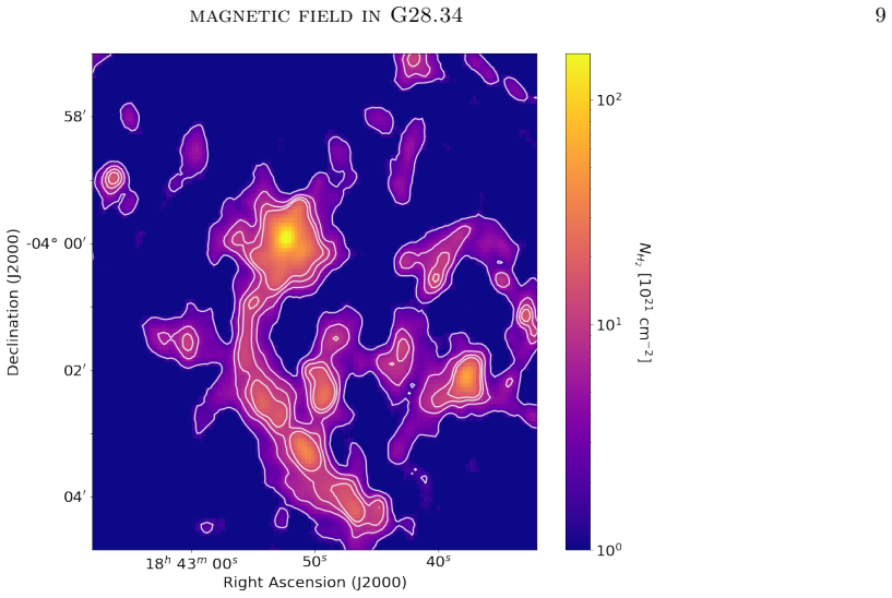
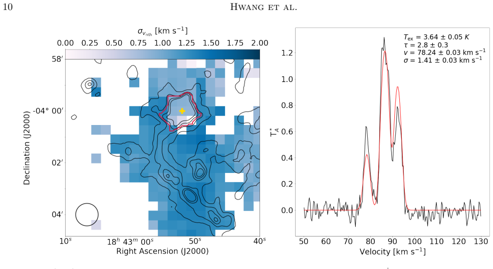
The two maps disagree in a striking way: the field direction on the two scales differs by 87 degrees, essentially perpendicular. To understand what that means, the team estimated the field strength using the standard Davis-Chandrasekhar-Fermi method: they combined the density of the gas, the spread of gas velocities from N2H+ molecules, and how tangled the field looks. They obtained plane-of-sky field strengths of about 50 to 430 microgauss. They then computed the mass-to-flux ratio, which compares the pull of gravity against the push of magnetic pressure. In the center, around the core, the ratio is above one, meaning gravity is winning and the region is collapsing.
The leading interpretation is that as the gas falls inward, it drags the magnetic field with it, rotating the field direction from clump scale to core scale. The authors also consider an alternative, an outflow from the forming star, and they state plainly that they cannot fully rule it out. Their own numbers come with large, honestly stated uncertainties, mainly because the field strength estimate depends on a calibration factor that could change the central mass-to-flux conclusion.
Extended reading notes
Core claim
The mean values of the JCMT and ALMA magnetic field directions are 24 and 117 degrees, with standard deviations of 19 and 32 degrees, respectively, indicating that the two magnetic field orientations are roughly perpendicular to one another with a mean angle difference of 87 degrees (Section 3.1). If the paper is correct, the field geometry in G28 P2 is scale-dependent: the clump-scale field (~2 to 0.3 pc) and the core-scale field (~0.3 to 0.02 pc) are nearly orthogonal, and the central region is magnetically supercritical, so gravitational collapse is the plausible cause of the reorientation.
Load-bearing premise
The correction factor Q = 0.28 (Liu et al. 2022), adopted in Equation (10) in place of the standard Q = 0.5, is what keeps the mean mass-to-flux ratio above unity (1.5 ± 0.5, Section 4.1). With Q = 0.5, the mean μΦ would be about 0.8 and the clump would be subcritical on average, weakening the collapse explanation for the perpendicular geometry. The paper states the factor-of-two effect on B but does not quantify that the supercritical-versus-subcritical conclusion, not just the field strength, hinges on this calibration.
Editorial analysis
A structured set of objections, weighed in public.
Assumptions & free parameters
free parameters (4)
- DCF correction factor Q =
0.28 (adopted from Liu et al. 2022; Ostriker et al. 2001 gives 0.5)
- Dust temperature for column density =
29 K (NH3 rotation temperature from Wang et al. 2008)
- Clump depth relative to radius =
1 R (equivalent radius, about 1 pc)
- Polarization selection thresholds =
I/ΔI ≥ 10, p/Δp ≥ 3, p < 20%; ALMA PI/σPI > 3
assumptions (7)
- domain assumption Polarized dust emission traces the plane-of-sky magnetic field via radiative alignment torques, with the field perpendicular to the polarization segments.
- domain assumption The DCF method converts angle dispersion and non-thermal velocity dispersion into field strength, with an order-unity correction factor Q.
- domain assumption Dust opacity model with κν0 = 0.1 cm2/g at 1 THz, β = 2, and gas-to-dust ratio 100.
- domain assumption The clump depth equals its equivalent radius R ≈ 1 pc (oblate geometry).
- domain assumption Kinetic temperature equals the NH3 rotation temperature, 29 K, for both the dust column (Eq. 7) and the N2H+ thermal correction (Eq. 9).
- domain assumption Distance to G28 is 4.8 kpc (Carey et al. 1998).
- domain assumption N2H+ hyperfine fitting yields the line-of-sight velocity dispersion of the dense gas.
Cite this review
Pith. "Pith review of The JCMT BISTRO-3 Survey: Variation of magnetic field orientations on parsec and sub-parsec scales in the massive star-forming region G28.34+0.06." pith.science (2026). https://pith.science/paper/4IMBPB2I
@misc{pith2026250514047,
  author       = {Pith},
  title        = {Pith review of: The JCMT BISTRO-3 Survey: Variation of magnetic field orientations on parsec and sub-parsec scales in the massive star-forming region G28.34+0.06},
  year         = {2026},
  howpublished = {\url{https://pith.science/paper/4IMBPB2I}},
  note         = {Machine review of arXiv:2505.14047}
}
read the original abstract
Magnetic fields play a significant role in star-forming processes on core to clump scales. We investigate magnetic field orientations and strengths in the massive star-forming clump P2 within the filamentary infrared dark cloud G28.34+0.06 using dust polarization observations made using SCUBA-2/POL-2 on the James Clerk Maxwell Telescope as part of the B-field In STar-forming Region Observations (BISTRO) survey. We compare the magnetic field orientations at the clump scale of ~2 parsecs from these JCMT observations with those at the core scale of ~0.2 parsecs from archival ALMA data, finding that the magnetic field orientations on these two different scales are perpendicular to one another. We estimate the distribution of magnetic field strengths, which range from 50 to 430 {\mu}G over the clump. The region forming the core shows the highest magnetic field strength. We also obtain the distribution of mass-to-flux ratios across the clump. In the region surrounding the core, the mass-to-flux ratio is larger than 1, which indicates the magnetic field strength is insufficient to support the region against gravitational collapse. Therefore, the change in the magnetic field orientation from clump to core scales may be the result of gravitational collapse, with the field being pulled inward along with the flow of material under gravity.
Figures


Figures from the paper (8 more)



Reference graph
Works this paper leans on
-
[1]
5 ZE @B1!E .XU Ŷ bǮ,/ uQ *oR@ ?gܙ HQ ąĈ < .nBk(\ \ x c!x _ǓH *֓ < b ) ; 8K(m _ @Jsк
thebibliography [1] 20pt to REFERENCES 6pt =0pt -12pt 10pt plus 3pt =0pt =0pt =1pt plus 1pt =0pt =0pt -12pt =13pt plus 1pt =20pt =13pt plus 1pt \@M =10000 =-1.0em =0pt =0pt 0pt =0pt =1.0em @enumiv\@empty 10000 10000 `\.\@m \@noitemerr \@latex@warning Empty `thebibliography' environment \@ifnextchar \@reference \@latexerr Missing key on reference command E...
2021
-
[2]
Andr \'e , P., Men'shchikov, A., Bontemps, S., et al.\ 2010, , 518, L102
2010
-
[3]
Bergin, E. A. & Langer, W. D.\ 1997, , 486, 316. doi:10.1086/304510
doi:10.1086/304510 1997
-
[4]
D., Linz, H., et al.\ 2020, , 904, 168
Beuther, H., Soler, J. D., Linz, H., et al.\ 2020, , 904, 168. doi:10.3847/1538-4357/abc019
-
[5]
Bino, G. & Basu, S.\ 2021, , 911, 15. doi:10.3847/1538-4357/abe6a4
-
[6]
Carey, S. J., Clark, F. O., Egan, M. P., et al.\ 1998, , 508, 721. doi:10.1086/306438
doi:10.1086/306438 1998
-
[7]
Carey, S. J., Feldman, P. A., Redman, R. O., et al.\ 2000, , 543, L157. doi:10.1086/317270
-
[8]
M., Zucconi, A., et al.\ 2002, , 565, 344
Caselli, P., Walmsley, C. M., Zucconi, A., et al.\ 2002, , 565, 344. doi:10.1086/324302
doi:10.1086/324302 2002
Show all 70 references
-
[9]
Chandrasekhar, S., & Fermi, E.\ 1953, , 118, 113
1953
-
[10]
L., Berry, D
Chapin, E. L., Berry, D. S., Gibb, A. G., et al.\ 2013, , 430, 2545. doi:10.1093/mnras/stt052
2013 doi
-
[11]
M., Troland, T
Crutcher, R. M., Troland, T. H., Lazareff, B., et al.\ 1999, , 514, L121
1999
-
[12]
M.\ 2004, , 292, 225
Crutcher, R. M.\ 2004, , 292, 225. doi:10.1023/B:ASTR.0000045021.42255.95
2004
-
[13]
M., Nutter, D
Crutcher, R. M., Nutter, D. J., Ward-Thompson, D., et al.\ 2004, , 600, 279. doi:10.1086/379705
2004 doi
-
[14]
J., Draper, P
Currie, M. J., Draper, P. W., Berry, D. S., et al.\ 2008, Astronomical Data Analysis Software and Systems XVII, 394, 650
2008
-
[15]
M., Wandelt, B., Heiles, C., et al.\ 2010, , 725, 466
Crutcher, R. M., Wandelt, B., Heiles, C., et al.\ 2010, , 725, 466. doi:10.1088/0004-637X/725/1/466
2010 doi
-
[16]
J., Berry, D
Currie, M. J., Berry, D. S., Jenness, T., et al.\ 2014, Astronomical Data Analysis Software and Systems XXIII, 485, 391
2014
-
[17]
Davis, L.\ 1951, Physical Review, 81, 890
1951
-
[18]
T., Friberg, P., Jenness, T., et al.\ 2013, , 430, 2534
Dempsey, J. T., Friberg, P., Jenness, T., et al.\ 2013, , 430, 2534
2013
-
[19]
M., Maury, A
Guillet, V., Girart, J. M., Maury, A. J., et al.\ 2020, , 634, L15. doi:10.1051/0004-6361/201937314
2020 doi
-
[20]
ascl:1305.010
Gildas Team\ 2013, Astrophysics Source Code Library. ascl:1305.010
2013
-
[21]
H.\ 1983, , 24, 267
Hildebrand, R. H.\ 1983, , 24, 267
1983
-
[22]
S., Bintley, D., Chapin, E
Holland, W. S., Bintley, D., Chapin, E. L., et al.\ 2013, , 430, 2513. doi:10.1093/mnras/sts612
2013 doi
-
[23]
Hull, C. L. H., Girart, J. M., Tychoniec, ., et al.\ 2017, , 847, 92. doi:10.3847/1538-4357/aa7fe9
2017 doi
-
[24]
doi:10.3847/1538-4357/abf3c4
Hwang, J., Kim, J., Pattle, K., et al.\ 2021, , 913, 85. doi:10.3847/1538-4357/abf3c4
2021 doi
-
[25]
doi:10.3847/1538-4357/ac99e0
Hwang, J., Kim, J., Pattle, K., et al.\ 2022, , 941, 51. doi:10.3847/1538-4357/ac99e0
2022 doi
- [26]
-
[27]
L., Berry, D
Jenness, T., Chapin, E. L., Berry, D. S., et al.\ 2013, Astrophysics Source Code Library, ascl:1310.007
2013
-
[28]
Jeong, I.-G., Kang, H., Jung, J., et al.\ 2019, Journal of Korean Astronomical Society, 52, 227
2019
-
[29]
L., et al.\ 2008, , 487, 993
Kauffmann, J., Bertoldi, F., Bourke, T. L., et al.\ 2008, , 487, 993
2008
-
[30]
M., Tang, Y.-W., & Ho, P
Koch, P. M., Tang, Y.-W., & Ho, P. T. P.\ 2012, , 747, 79
2012
-
[31]
M., Tang, Y.-W., Ho, P
Koch, P. M., Tang, Y.-W., Ho, P. T. P., et al.\ 2018, , 855, 39. doi:10.3847/1538-4357/aaa4c1
2018 doi
-
[32]
M., Tang, Y.-W., Ho, P
Koch, P. M., Tang, Y.-W., Ho, P. T. P., et al.\ 2022, , 940, 89. doi:10.3847/1538-4357/ac96e3
2022 doi
-
[33]
Kumar, M. S. N., Palmeirim, P., Arzoumanian, D., et al.\ 2020, , 642, A87. doi:10.1051/0004-6361/202038232
2020 doi
-
[34]
& Hoang, T.\ 2007, , 378, 910
Lazarian, A. & Hoang, T.\ 2007, , 378, 910
2007
-
[35]
B., Dale, J
Lin, Y., Liu, H. B., Dale, J. E., et al.\ 2017, , 840, 22. doi:10.3847/1538-4357/aa6c67
2017 doi
-
[36]
doi:10.3847/1538-4357/ab9087
Liu, J., Zhang, Q., Qiu, K., et al.\ 2020, , 895, 142. doi:10.3847/1538-4357/ab9087
2020 doi
-
[37]
doi:10.3847/1538-4357/ac0cec
Liu, J., Zhang, Q., Commer c on, B., et al.\ 2021, , 919, 2, 79. doi:10.3847/1538-4357/ac0cec
2021 doi
-
[38]
doi:10.3389/fspas.2022.943556
Liu, J., Zhang, Q., & Qiu, K.\ 2022, Frontiers in Astronomy and Space Sciences, 9, 943556. doi:10.3389/fspas.2022.943556
2022
-
[39]
doi:10.3847/1538-4357/ad3105
Liu, J., Zhang, Q., Lin, Y., et al.\ 2024, , 966, 120. doi:10.3847/1538-4357/ad3105
2024 doi
-
[40]
doi:10.3847/1538-4357/ab0958
Liu, J., Qiu, K., Berry, D., et al.\ 2019, , 877, 43. doi:10.3847/1538-4357/ab0958
2019 doi
-
[41]
S., Juvela, M., et al.\ 2018, , 859, 151
Liu, T., Li, P. S., Juvela, M., et al.\ 2018, , 859, 151. doi:10.3847/1538-4357/aac025
2018 doi
-
[42]
T., Bell, G
Mairs, S., Dempsey, J. T., Bell, G. S., et al.\ 2021, , 162, 191. doi:10.3847/1538-3881/ac18bf
2021 doi
-
[43]
A., Whitworth, A
Marsh, K. A., Whitworth, A. P., Lomax, O., et al.\ 2017, , 471, 2730. doi:10.1093/mnras/stx1723
2017 doi
-
[44]
Motte, F., & Andr \'e , P.\ 2001, , 365, 440
2001
-
[45]
P., Waters, B., Schiebel, D., et al.\ 2007, Astronomical Data Analysis Software and Systems XVI, 376, 127
McMullin, J. P., Waters, B., Schiebel, D., et al.\ 2007, Astronomical Data Analysis Software and Systems XVI, 376, 127
2007
-
[46]
C., & Spitzer, L.\ 1976, , 210, 326
Mouschovias, T. C., & Spitzer, L.\ 1976, , 210, 326
1976
-
[47]
Mouschovias, T. C. & Ciolek, G. E.\ 1999, The Origin of Stars and Planetary Systems, 540, 305
1999
- [48]
-
[49]
& Nakamura, T.\ 1978, , 30, 671
Nakano, T. & Nakamura, T.\ 1978, , 30, 671
1978
-
[50]
C., Stone, J
Ostriker, E. C., Stone, J. M., & Gammie, C. F.\ 2001, , 546, 980
2001
-
[51]
doi:10.1051/0004-6361/201220500
Palmeirim, P., Andr \'e , P., Kirk, J., et al.\ 2013, , 550, A38. doi:10.1051/0004-6361/201220500
2013 doi
- [52]
-
[53]
Pety, J.\ 2005, SF2A-2005: Semaine de l'Astrophysique Francaise, 721
2005
-
[54]
M.\ 2016, , 591, A19
Pillai, T., Kauffmann, J., Wiesemeyer, H., & Menten, K. M.\ 2016, , 591, A19
2016
-
[55]
doi:10.3847/1538-4357/abcc6c
Pattle, K., Lai, S.-P., Di Francesco, J., et al.\ 2021, , 907, 88. doi:10.3847/1538-4357/abcc6c
2021 doi
-
[56]
& Fissel, L.\ 2019, Frontiers in Astronomy and Space Sciences, 6, 15
Pattle, K. & Fissel, L.\ 2019, Frontiers in Astronomy and Space Sciences, 6, 15. doi:10.3389/fspas.2019.00015
2019
-
[57]
doi:10.3847/2041-8213/aac771
Pattle, K., Ward-Thompson, D., Hasegawa, T., et al.\ 2018, , 860, L6. doi:10.3847/2041-8213/aac771
2018 doi
-
[58]
doi:10.3847/1538-4357/aa80e5
Pattle, K., Ward-Thompson, D., Berry, D., et al.\ 2017, , 846, 122. doi:10.3847/1538-4357/aa80e5
2017 doi
-
[59]
Planck Collaboration, Ade, P. A. R., Aghanim, N., et al.\ 2015, , 576, A104. doi:10.1051/0004-6361/201424082
2015 doi
-
[60]
Planck Collaboration, Ade, P. A. R., Aghanim, N., et al.\ 2016, , 586, A138. doi:10.1051/0004-6361/201525896
2016 doi
-
[61]
W., Reipurth, B., & Bally, J.\ 2003, , 125, 2108
Pound, M. W., Reipurth, B., & Bally, J.\ 2003, , 125, 2108. doi:10.1086/368138
2003 doi
-
[62]
W., Pineda, J
Rosolowsky, E. W., Pineda, J. E., Kauffmann, J., et al.\ 2008, , 679, 1338. doi:10.1086/587685
2008 doi
-
[63]
Roy, A., Andr \'e , P., Palmeirim, P., et al.\ 2014, , 562, A138
2014
-
[64]
M., Padovani, M., et al.\ 2021, , 915, L10
Sanhueza, P., Girart, J. M., Padovani, M., et al.\ 2021, , 915, L10. doi:10.3847/2041-8213/ac081c
2021 doi
-
[65]
D., Hennebelle, P., Martin, P
Soler, J. D., Hennebelle, P., Martin, P. G., et al.\ 2013, , 774, 128
2013
-
[66]
L.\ 2015, , The Critical Density and the Effective Excitation Density of Commonly Observed Molecular Dense Gas Tracers, 127, 949, 299
Shirley, Y. L.\ 2015, , The Critical Density and the Effective Excitation Density of Commonly Observed Molecular Dense Gas Tracers, 127, 949, 299. doi:10.1086/680342
2015 doi
-
[67]
M., Peretto, N., et al.\ 2019, , 878, 10
Tang, Y.-W., Koch, P. M., Peretto, N., et al.\ 2019, , 878, 10. doi:10.3847/1538-4357/ab1484
2019 doi
-
[68]
doi:10.1086/524949
Wang, Y., Zhang, Q., Pillai, T., et al.\ 2008, , 672, L33. doi:10.1086/524949
2008 doi
-
[69]
Ward-Thompson, D., Pattle, K., Bastien, P., et al.\ 2017, , 842, 66
2017
-
[70]
M., et al.\ 2014, , 792, 116
Zhang, Q., Qiu, K., Girart, J. M., et al.\ 2014, , 792, 116. doi:10.1088/0004-637X/792/2/116
2014 doi
Reviewed August 7, 2026 · model on record in the stance chip above.
Discussion (0). Continue with ORCID to comment.