REVIEW 5 major objections 4 minor 35 references
Conservation Laws with Discontinuous Gradient-Dependent Flux: the Unstable Case
T0 review · 5 major / 4 minor · reviewed 2026-08-12 · deepseek-v4-flash
Pith's one-line read Infinitely many admissible solutions arise even from zero data in the unstable f>g case.
desk verdict Genuinely new treatment of the unstable f>g case with a correct infinite-non-uniqueness example, but Theorem 3.1's proof has real gaps: the 'entirely similar' local cases (especially 4B) and the finite-restart claim are not established as written. read the letter →
The pith
A machine-rendered reading of the paper's core claim, the machinery that carries it, and where it could break.
The reading
What carries the argument
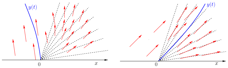
The load-bearing object is the interface curve x=y(t) separating the region where theta=1 (flux f) from the region where theta=0 (flux g), together with the Rankine-Hugoniot speed function H(t,x)=(f(u♭(t,x−))−g(u♯(t,x+)))/(u♭−u♯) that must equal dot y(t). Existence and uniqueness of the interface is reduced to a discontinuous ordinary differential equation dot y=H(t,y), solved by gluing two auxiliary solutions u♭ and u♯ of the single-flux conservation laws (2.7) and (2.18). Uniqueness of the interface uses the theory of discontinuous ODEs: in Case 2A the coefficient H is shown to have bounded directional variation on a cone Γ, so Bressan's uniqueness theorem applies, while in Case 2B a Picard contraction on a wedge Wε2 is proved with the aid of a lemma comparing values of a decreasing function along two curves. The global solution is then assembled by restarting the construction at each time when two interfaces meet, which reduces the interface count and can happen only finitely often.
What would settle it
Compute or simulate the interface ODE (4.6) for the fluxes f(u)=$u^{2}$/2+1 and g(u)=$u^{2}$/2 and look for two different admissible interface curves y(t) through the origin within the cone Γ of (4.11); if two exist, uniqueness in Case 2A fails. More directly, check numerically whether H in (4.5) has bounded directional variation on that cone for a profile where u♯ contains a compression wave; a curve along which H has infinite variation would break the cited uniqueness theorem.
Extended reading notes
Core claim
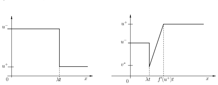
On the paper's own terms, the discovery is that the unstable gradient-dependent flux law (1.1)-(1.2) has a definite solution theory if the right selection criterion is imposed. For any Riemann data, an admissible solution is constructed case by case from shocks and centered rarefactions, with the switching set theta determined by the sign of u_x. Because any point of a constant profile can be read as a local maximum, zero initial data yields a continuum of admissible triangular spike solutions; new spikes can be nucleated at arbitrary times at any point where a decreasing solution is smooth. Restricting to piecewise monotone initial data with a prescribed interface set, the paper constructs a global piecewise monotone admissible solution for all t>=0, with interfaces governed by the discontinuous Rankine-Hugoniot ODE (4.6). The uniqueness statement is conditional: among all admissible solutions, exactly one has the minimal possible number of interfaces at every time, and this is the solution constructed.
Load-bearing premise
The global uniqueness proof rests on the assertion that the interface speed H has bounded directional variation on the cone Γ in Case 2A and on the dismissal of Cases 3 and 4B as entirely similar to Case 2; if either assertion fails, the constructed minimal-interface solution may not be the only one, or may not exist.
Editorial extensions
If this is right
- The Riemann problem for (1.1)-(1.2) is solvable in all four combinations of θ−, θ+; solvability is explicit, with shock speeds given by tangent-line constructions on the graph of f.
- Any smooth decreasing region of a solution is a nucleation site: two new spikes can appear at any time and then persist, so the set of admissible solutions is at least one-dimensional even from simple data.
- For piecewise monotone initial data, a global admissible solution exists for all t≥0 and its total variation does not increase in time, because characteristics impinge on every interface from both sides.
- Uniqueness is restored, within the class considered, by the minimal-interface rule: at each shock interaction the solution with the fewest interfaces is the one the construction selects.
Reading between the lines
- If f and g cross, the model should switch from well-posed (stable, f<g) to ill-posed (unstable, f>g) as the density u crosses the intersection; the minimal-interface rule gives a plausible selection principle in the unstable regime but is not derived from any physical or entropic limit.
- The spike-nucleation mechanism suggests that any numerical or viscous regularization that keeps the transition layer narrow will effectively choose one of the infinitely many admissible solutions; measuring which spike locations are selected under a given regularization would test the modeling value of the minimal-interface criterion.
- The same interface-ODE machinery could be applied to systems with two convex fluxes selected by the gradient of a second variable, e.g. two-phase or hysteretic models, whenever the unstable sign condition holds.
Editorial analysis
A structured set of objections, weighed in public.
Referee Report
Summary. The paper studies the scalar conservation law u_t + (θ(u_x)f(u) + (1-θ(u_x))g(u))_x = 0 in the 'unstable' case f > g, with f and g strictly convex. It constructs Lax-admissible solutions to the Riemann problem in four separate cases, gives an explicit non-uniqueness example for zero initial data (Example 2.1), introduces a class of piecewise monotone solutions with interfaces, and states Theorem 3.1 claiming global existence for all t >= 0 and uniqueness under an additional minimal-interface rule. The proof is based on local generalized Riemann problems whose interface curves are determined by discontinuous ODEs, invoking uniqueness results from [9].
Significance. If completed, the paper would show that even in a scalar one-dimensional conservation law, Lax admissibility alone does not select a unique solution, and that a natural 'minimal interfaces' criterion can restore uniqueness in a piecewise monotone class. The explicit family of triangular spike solutions in Example 2.1 is simple, fully verified, and convincing; the local Case 2B construction through a contractive Picard operator is a substantial piece of analysis; and the paper is honest about the conditional nature of the uniqueness statement, especially in Remark 2.3. However, the global theorem is only as strong as the omitted local cases and the interaction argument, which are not proved in the manuscript as written.
major comments (5)
- [Section 4, Case 4B] The uniqueness of the pair of interface curves (y,z) is asserted by saying that 'the existence and uniqueness of the solution is proved by the same arguments as in Case 2 and Case 3', but Case 2 provides only a scalar contraction argument for one curve, and the quoted uniqueness theorem [9] is for a scalar discontinuous ODE. For the system (4.34)-(4.37), the two curves enclose a centered f-rarefaction and interact with both auxiliary solutions u♭ and u♯, so a genuine vector-valued discontinuous-ODE theorem or a two-curve contraction proof is required; none is stated or proved.
- [Section 4, Case 3] The interface ODE (4.6), (4.33) is dismissed with 'the proof ... is achieved by the same arguments as in Case 2. We thus omit the details.' Here the flux values are g on the left and f on the right, the monotonicity of the auxiliary solutions is different from Case 2, and the tangency construction in Lemma 2.2 is not symmetric with respect to exchanging u− and u+. A detailed verification of bounded directional variation, or another complete uniqueness argument, is needed for this case; omitting it leaves the global construction incomplete.
- [Section 4, Case 2A] After (4.11), the claim that H has bounded directional variation on the cone Γ and hence the theorem of [9] applies is justified only by the sentence 'This is obvious ...'. The reader needs an explicit estimate of the total variation of t ↦ u♭(t,x(t)) and t ↦ u♯(t,x(t)) for arbitrary Lipschitz curves with |ẋ(t)-λ| ≤ 2ε, including a justification that the curves do not cross the rarefaction fan boundary in a way that produces multiple oscillations. Boundedness of the BV norms of u♭ and u♯ alone does not automatically control composition with an arbitrary Lipschitz curve of positive speed.
- [Section 4, item 6] The statement that at the first interaction time 'the number of interfaces decreases at least by one' is asserted without proof. This is not automatic: a non-interface g-shock can meet an interface, and local Riemann data with θ− = θ+ = 0 and u− < u+ are handled by Case 4B, whose minimal solution creates two new interfaces. The proof must analyze all collision patterns and show that the minimal-interface rule still yields a strictly smaller interface count after the interaction, or else the finite-restarting argument fails.
- [Theorem 3.1] The uniqueness half of Theorem 3.1 is conditional on a 'minimum number of interfaces at each point of shock interaction' rule that is stated only informally. Since Remark 2.3 exhibits two admissible Riemann solutions with different interface counts, and Example 2.1 shows non-uniqueness for smooth data, the theorem's uniqueness claim is not a statement about the equation alone. The manuscript should formalize the selection rule and prove that it is well-defined, for instance by showing that ties cannot occur or by specifying how ties are broken.
minor comments (4)
- [Section 4, Case 2A] The condition is written as u− > u∗, while the corresponding Riemann case in Section 2, Case 2A, uses u∗ ≤ u−; the boundary case u− = u∗ should be treated explicitly.
- [Section 4, Case 2B proof] The paragraph beginning '5.' appears to be a numbering artifact; it should be integrated into the preceding proof.
- [Definition 3.1(iii)] The distributional formulation splits the integral over {θ = 1} and {θ = 0}; since θ is only defined a.e., the manuscript should specify the representative of θ used to define these sets.
- [Example 2.1] In (2.4), θ = 1 is assigned for x − x0 < √2 t, which includes the region x < x0 where u is constant; this is consistent with Definition 1.1 but deserves a remark because θ is not determined by the gradient there.
Circularity Check
No significant circularity: the minimal-interface rule is an explicit selection criterion, and the cited ODE uniqueness theorem is independent published support.
full rationale
The paper's derivation chain is not circular. The Riemann problem solutions in Section 2 are constructed by explicit verification of the Rankine-Hugoniot and Lax admissibility conditions, and the non-uniqueness example (Example 2.1) is a direct family of piecewise-smooth functions checked against the PDE. Theorem 3.1 does not claim the equation alone determines a unique solution; instead, it states uniqueness only under the explicitly imposed minimal-interface condition. That condition is a selection rule, not a hidden input disguised as an output; the paper openly acknowledges alternative admissible solutions (Remark 2.3) and states that the choice is made by preference for the least number of interfaces. The proof's reliance on [9] is not circular: [9] is a published general theorem on discontinuous ODEs with stated hypotheses that do not include the present result, and the authors also provide a self-contained contraction argument in Case 2B and a proof of Lemma 4.1. The remaining appeals to 'entirely similar techniques' (Cases 3 and 4B), the sketched verification of bounded directional variation in Case 2A, and the claim that each interaction reduces the interface count are potential completeness or correctness gaps, but they are not reductions of the conclusion to the hypothesis. No fitted parameter is renamed as a prediction, and no known result is repackaged under new coordinates as if it were new.
Assumptions & free parameters
assumptions (6)
- domain assumption f and g are C^2, strictly convex, and f(u) > g(u) for all u in R
- domain assumption Initial data is piecewise monotone with finitely many monotonicity intervals, plus an assigned interface set
- domain assumption Lax admissibility conditions (1.13) are the correct entropy selection
- standard math Bressan's uniqueness theorem for discontinuous ODEs [9] holds and applies to the interface equation (4.6)
- standard math Standard theory of scalar conservation laws with strictly convex flux provides entropy solutions used as building blocks
- ad hoc to paper The minimal-interface rule is well-defined and always yields a unique continuation
Cite this review
Pith. "Pith review of Conservation Laws with Discontinuous Gradient-Dependent Flux: the Unstable Case." pith.science (2026). https://pith.science/paper/4MJCOEEV
@misc{pith2026241113444,
  author       = {Pith},
  title        = {Pith review of: Conservation Laws with Discontinuous Gradient-Dependent Flux: the Unstable Case},
  year         = {2026},
  howpublished = {\url{https://pith.science/paper/4MJCOEEV}},
  note         = {Machine review of arXiv:2411.13444}
}
abstract
The paper is concerned with a scalar conservation law with discontinuous gradient-dependent flux. Namely, the flux is described by two different functions $f(u)$ or $g(u)$, when the gradient $u_x$ of the solution is positive or negative, respectively. We study here the unstable case where $f(u)>g(u)$ for all $u\in {\mathbb R}$. Assuming that both $f$ and $g$ are strictly convex, solutions to the Riemann problem are constructed. Even for a smooth initial data, examples show that the Cauchy problem can have infinitely many solutions. For an initial data which is piecewise monotone, i.e., increasing or decreasing on a finite number of intervals, a solution can be constructed globally in time. It is proved that such solution is unique under the additional requirement that the number of interfaces, where the flux switches between $f$ and $g$, remains as small as possible.
Figures


Figures from the paper (12 more)






Reference graph
Works this paper leans on
-
[2]
D. Amadori, A. Bressan and W. Shen. Conservation laws with discontinuous gradient- dependent flux: the stable case. Preprint 2024
work page 2024
-
[9]
A. Bressan. Unique solutions for a class of discontinuous differential equations. Proc. Amer. Math. Soc. , 104 (1988), 772–778
work page 1988
-
[1]
Adimurthi, S. Mishra and G. D. Veerappa Gowda. Optimal entropy solutions for con- servation laws with discontinuous flux-functions.J. Hyperbolic Differ. Equat., 2 (2005), 783–837
work page 2005
-
[3]
F. Ancona and M. T. Chiri. Well-posedness of conservation laws for production lines with discontinuous flux in the unknown. Preprint, University of Padova, 2024
work page 2024
-
[4]
B. Andreianov. New approaches to describing admissibility of solutions of scalar con- servation laws with discontinuous flux. ESAIM: Proc. and Surveys , 50 (2015), 40–65
work page 2015
-
[5]
B. Andreianov, K. H. Karlsen, and N. H. Risebro. A theory of L1-dissipative solvers for scalar conservation laws with discontinuous flux. Arch. Ration. Mech. Anal. , 201 (2011), 27–86
work page 2011
-
[6]
B. Andreianov and D. Mitrovi´ c. Entropy conditions for scalar conservation laws with discontinuous flux revisited. Ann. Inst. H. Poincar´ e Anal. Non Lin´ eaire, 32 (2015), 1307–1335
work page 2015
-
[7]
E. Audusse and B. Perthame. Uniqueness for scalar conservation laws with discon- tinuous flux via adapted entropies. Proc. Roy. Soc. Edinburgh , Sect. A, 135 (2005), 253–265
work page 2005
Show all 35 references
-
[8]
Bachmann and J
F. Bachmann and J. Vovelle. Existence and uniqueness of entropy solution of scalar conservation laws with a flux function involving discontinuous coefficients.Comm. Par- tial Differential Equations , 31 (2006), 371–395
2006
-
[10]
A. Bressan. Hyperbolic systems of conservation laws. The one dimensional Cauchy problem. Oxford University Press, 2000
2000
-
[11]
Bressan, G
A. Bressan, G. Guerra and W. Shen. Vanishing viscosity solutions for conservation laws with regulated flux. J. Differential Equations , 266 (2019), 312–351
2019
-
[12]
Bressan and W
A. Bressan and W. Shen. Uniqueness for discontinuous ODE and conservation laws. Nonlinear Anal., 34 (1998), 637–652
1998
-
[13]
Bul ´ ı˘ cek, P
M. Bul ´ ı˘ cek, P. Gwiazda, J. M´ alek and A.´Swierczewska-Gwiazda. On scalar hyperbolic conservation laws with a discontinuous flux. Math. Models Methods Appl. Sci. , 21 (2011), 89–113. 25
2011
-
[14]
Bul ´ ı˘ cek, P
M. Bul ´ ı˘ cek, P. Gwiazda and A.´Swierczewska-Gwiazda. Multi-dimensional scalar con- servation laws with fluxes discontinuous in the unknown and the spatial variable. Math. Models Methods Appl. Sci. , 23 (2013), 407–439
2013
-
[15]
Bul ´ ı˘ cek, P
M. Bul ´ ı˘ cek, P. Gwiazda and A.´Swierczewska-Gwiazda. On unified theory for scalar conservation laws with fluxes and sources discontinuous with respect to the unknown. J. Differential Equations , 262 (2017), 313–364
2017
-
[16]
Corli and H
A. Corli and H. Fan. Hysteresis and stop-and-go waves in traffic flows. Math. Models Methods Appl. Sci. , 29 (2019), 2637–2678
2019
-
[17]
G. M. Coclite and N. H. Risebro. Conservation laws with time dependent discontinuous coefficients. SIAM J. Math. Anal. , 36 (2005), 1293–1309
2005
-
[18]
S. Diehl. On scalar conservation laws with point source and discontinuous flux function. SIAM J. Math. Anal. , 26 (1995), 1425–1451
1995
-
[19]
T. Gimse. Conservation laws with discontinuous flux functions. SIAM J. Math. Anal. , 24 (1993), 279–289
1993
-
[20]
Gimse and N
T. Gimse and N. H. Risebro. Riemann problems with a discontinuous flux function. Third International Conference on Hyperbolic Problems , (Uppsala, 1990), 488–502. Studentlitteratur, Lund, 1991
1990
-
[21]
Gimse and N
T. Gimse and N. H. Risebro. Solution of the Cauchy problem for a conservation law with discontinuous flux function. SIAM J. Math. Anal. , 23 (1992), 635–648
1992
-
[22]
Guerra and W
G. Guerra and W. Shen. Backward Euler approximations for conservation laws with discontinuous flux. SIAM J. Math. Anal. , 51 (2019), 3112–3144
2019
-
[23]
H. Fan. Conservation laws with hysteretic fluxes.J. Differential Equations, 394 (2024), 1–30
2024
-
[24]
R. A. Klausen and N. H. Risebro. Stability of conservation laws with discontinuous coefficients. J. Differential Equations , 157 (1999), 41–60
1999
-
[25]
Klingenberg and N
C. Klingenberg and N. H. Risebro. Convex conservation laws with discontinuous co- efficients, existence, uniqueness and asymptotic behavior. Comm. Partial Differential Equations, 20 (1995), 1959–1990
1995
-
[26]
S. Mishra. Convergence of upwind finite difference schemes for a scalar conservation law with indefinite discontinuities in the flux function. SIAM J. Numer. Anal. , 43 (2005), 559–577
2005
-
[27]
E. Y. Panov. Existence and strong pre-compactness properties for entropy solutions of a first-order quasilinear equation with discontinuous flux. Arch. Ration. Mech. Anal. , 195 (2010), 643–673
2010
-
[28]
E. Y. Panov. On entropy solutions of scalar conservation laws with discontinuous flux. Arch. Ration. Mech. Anal. , 247 (2023), paper No. 78, 40 pp
2023
-
[29]
Seguin and J
N. Seguin and J. Vovelle. Analysis and approximation of a scalar conservation law with a flux function with discontinuous coefficients. Math. Models Methods Appl. Sci. , 13 (2003), 221–257. 26
2003
-
[30]
W. Shen. Slow erosion with rough geological layers. SIAM J. Math. Anal. 47 (2015), 3116–3150
2015
-
[31]
W. Shen. On the Cauchy problems for polymer flooding with gravitation. J. Differen- tial Equations 261 (2016), 627–653
2016
-
[32]
W. Shen. Global Riemann solvers for several 3 × 3 systems of conservation laws with degeneracies. Math. Models Methods Appl. Sci. , 28 (2018), 1599–1626
2018
-
[33]
J. D. Towers. Convergence of a difference scheme for conservation laws with a discon- tinuous flux. SIAM J. Numer. Anal. , 38 (2000), 681–698
2000
-
[34]
J. D. Towers. A splitting algorithm for L WR traffic models with flux discontinuous in the unknown. J. Comput. Phys. , 421 (2020), 109722, 30 pp
2020
-
[35]
Treiterer and J
J. Treiterer and J. Myers. The hysteresis phenomenon in traffic flow. In Proceedings of the Sixth Symposium on Transportation and Traffic Theory , D.J. Buckley, editor, (1974), pp. 13–38. 27
1974
Reviewed August 12, 2026 · model on record in the stance chip above.
Discussion (0). Continue with ORCID to comment.