Stochastic Convergence Analysis for Large-Scale Linear Discrete Ill-posed Problems
Pith reviewed 2026-05-20 00:04 UTC · model grok-4.3
The pith
Polynomial upper bound on generalized eigenvalues allows stochastic error bounds for weighted Tikhonov regularization in large-scale ill-posed problems.
A machine-rendered reading of the paper's core claim, the machinery that carries it, and where it could break.
Core claim
Under a polynomial upper-bound assumption on the generalized eigenvalues of the discrete forward operator, stochastic error bounds are derived for weighted Tikhonov regularization. Expectation bounds are obtained for independent zero-mean bounded-variance noise and high-probability bounds for independent sub-Gaussian noise. The analysis provides an a priori parameter-choice rule and an adaptive strategy for large-scale computation.
What carries the argument
Polynomial upper-bound assumption on the generalized eigenvalues of the discrete forward operator, which controls the decay and enables derivation of the explicit stochastic error rates and parameter rules.
If this is right
- An a priori parameter-choice rule follows directly from the error bounds and achieves the predicted convergence rates.
- An adaptive strategy is suggested that remains effective for large-scale computation without explicit knowledge of the noise level.
- The derived bounds apply in expectation to zero-mean bounded-variance noise and with high probability to sub-Gaussian noise.
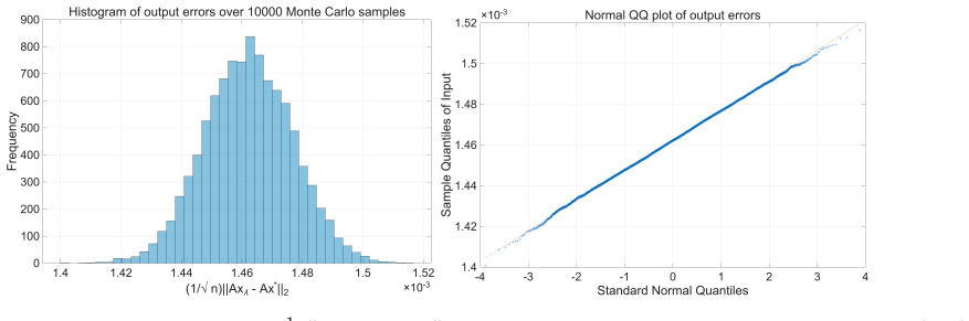
- Numerical experiments confirm that the parameter selected by the rule is nearly optimal and that the adaptive method works in practice.
Where Pith is reading between the lines
- For discretizations whose eigenvalues are known to decay polynomially, the a priori rule could replace more expensive parameter-tuning procedures such as cross-validation.
- The high-probability bounds could support uncertainty quantification by providing explicit probabilistic guarantees on reconstruction accuracy.
- The same assumption and bounding technique might extend to other regularization schemes or to continuous operator settings if analogous eigenvalue control holds.
Load-bearing premise
The generalized eigenvalues of the discrete forward operator are upper-bounded by a polynomial in their ordering index.
What would settle it
Compute the generalized eigenvalues on a discretization of an ill-posed problem; if they violate the polynomial upper bound yet the observed reconstruction error with the a priori parameter still matches the predicted rate, or if they obey the bound but the error exceeds the bound, the claim is falsified.
Figures


read the original abstract
We study weighted Tikhonov regularization for large-scale linear discrete ill-posed problems with random noise. Under a polynomial upper-bound assumption on the generalized eigenvalues of the discrete forward operator, we derive stochastic error bounds for two noise models: expectation bounds for independent zero-mean bounded-variance noise, and high-probability bounds for independent sub-Gaussian noise. The analysis yields an a priori parameter-choice rule and suggests an adaptive strategy suitable for large-scale computation. Numerical experiments support the theory and show that the predicted parameter is nearly optimal and that the adaptive method is effective in practice.
Editorial analysis
A structured set of objections, weighed in public.
Referee Report
Summary. The manuscript analyzes stochastic error bounds for weighted Tikhonov regularization of large-scale linear discrete ill-posed problems. Under the assumption that the generalized eigenvalues of the discrete forward operator satisfy a polynomial upper bound λ_j ≤ C j^{-α} (α > 0), expectation bounds are derived for independent zero-mean bounded-variance noise and high-probability bounds for independent sub-Gaussian noise. The analysis produces an a priori parameter-choice rule and an adaptive strategy for large-scale settings. Numerical experiments on standard test problems are reported to illustrate the theory and indicate that the predicted parameter is nearly optimal while the adaptive method is effective.
Significance. If the polynomial eigenvalue-decay assumption holds for the operators arising in typical large-scale discretizations, the derived stochastic bounds and the associated a priori/adaptive parameter rules would constitute a useful contribution to regularization theory for random-noise inverse problems. The explicit treatment of both expectation and high-probability settings, together with a computationally feasible adaptive strategy, strengthens the practical relevance. The numerical illustrations provide initial evidence of performance, but the overall significance remains conditional on verification of the modeling hypothesis.
major comments (1)
- [Numerical experiments] The central theorems (preceding the main results) and the subsequent a priori parameter rule rest on the polynomial upper-bound assumption λ_j ≤ C j^{-α}. The numerical experiments section reports results on standard discretizations of integral operators yet contains no computation, table, or plot of the observed generalized eigenvalue (or singular-value) decay that would confirm the assumption holds with the stated form for the concrete matrices employed. Without this check, the claim that the predicted parameter is “nearly optimal” and that the experiments support the derived rates rests on an unverified modeling hypothesis rather than on the actual operators tested.
Simulated Author's Rebuttal
We thank the referee for the careful review and constructive feedback on our manuscript. We address the major comment point by point below.
read point-by-point responses
-
Referee: [Numerical experiments] The central theorems (preceding the main results) and the subsequent a priori parameter rule rest on the polynomial upper-bound assumption λ_j ≤ C j^{-α}. The numerical experiments section reports results on standard discretizations of integral operators yet contains no computation, table, or plot of the observed generalized eigenvalue (or singular-value) decay that would confirm the assumption holds with the stated form for the concrete matrices employed. Without this check, the claim that the predicted parameter is “nearly optimal” and that the experiments support the derived rates rests on an unverified modeling hypothesis rather than on the actual operators tested.
Authors: We agree that including a verification of the polynomial eigenvalue decay assumption for the specific test problems would make the numerical section more convincing and directly link the experiments to the theoretical assumptions. In the revised version of the manuscript, we will add a new figure showing the decay of the generalized eigenvalues for the discretizations used in the experiments (such as those from the Regularization Tools package). This will demonstrate that the assumption λ_j ≤ C j^{-α} holds for suitable α > 0, thereby justifying the application of our derived bounds and parameter-choice rules to these problems. revision: yes
Circularity Check
No significant circularity; derivation proceeds from explicit assumptions to derived bounds
full rationale
The paper explicitly invokes a polynomial upper-bound assumption on the generalized eigenvalues of the discrete forward operator as the foundation for deriving stochastic error bounds (expectation bounds under bounded-variance noise and high-probability bounds under sub-Gaussian noise) and the associated a priori parameter-choice rule. No quoted steps reduce these bounds or rules back to fitted parameters, self-citations, or input data by construction. The analysis is forward from the stated modeling hypothesis and noise models to the convergence results, with numerical experiments presented only as empirical support rather than definitional inputs. This constitutes a standard assumption-based theoretical derivation without load-bearing circular reductions.
Axiom & Free-Parameter Ledger
axioms (1)
- domain assumption Polynomial upper-bound assumption on the generalized eigenvalues of the discrete forward operator
Reference graph
Works this paper leans on
-
[1]
H. Andrews and B. Hunt.Digital Image Restoration. Prentice Hall, Englewood Cliffs, NJ, 1977
work page 1977
-
[2]
D. Bianchi, M. Donatelli, D. Furchí, and L. Reichel. Convergence analysis and parameter estima- tion for the iterated arnoldi–tikhonov method.Numerische Mathematik, 157:749–779, 2025
work page 2025
-
[3]
A. F. Boden, D. C. Redding, R. J. Hanisch, and J. Mo. Massively parallel spatially-variant maximum likelihood restoration of hubble space telescope imagery.Journal of the Optical Society of America A, 13:1537–1545, 1996
work page 1996
-
[4]
N. K. Bose and K. J. Boo. High-resolution image reconstruction with multisensors.International Journal of Imaging Systems and Technology, 9:294–304, 1998
work page 1998
-
[5]
A. Buccini, S. Gazzola, L. Onisk, M. Pasha, and L. Reichel. Projected iterated tikhonov in general form with adaptive choice of the regularization parameter.Numerical Algorithms, 100:1617–1637, 2025
work page 2025
-
[6]
T. M. Buzug.Computed Tomography. Springer, Berlin, 2008
work page 2008
-
[7]
Z. Chen, R. Tuo, and W. Zhang. Stochastic convergence of a nonconforming finite element method for the thin plate spline smoother for observational data.SIAM Journal on Numerical Analysis, 56:635–659, 2018
work page 2018
- [8]
-
[9]
J. Chung and S. Gazzola. Computational methods for large-scale inverse problems: A survey on hybrid projection methods.SIAM Review, 66(2):205–284, 2024
work page 2024
-
[10]
J. Chung and K. Palmer. A hybrid LSMR algorithm for large-scale tikhonov regularization.SIAM Journal on Scientific Computing, 37(5):S562–S580, 2015. 19 (a) Convergence history of the adaptive reg- ularization parameterλ k forδ= 0.01and n= 10000. (b) Convergence history of the adaptive reg- ularization parameterλ k forδ= 0.001and n= 32400. (c) The output e...
work page 2015
-
[11]
J. Chung and A. K. Saibaba. Generalized hybrid iterative methods for large-scale bayesian inverse problems.SIAM Journal on Scientific Computing, 39(5):S24–S46, 2017
work page 2017
-
[12]
C. L. Epstein.Introduction to the Mathematics of Medical Imaging. SIAM, Philadelphia, 2nd edition, 2007
work page 2007
-
[13]
S. Gazzola, P. C.Hansen, and J. G. Nagy. IR Tools: A MATLAB package of iterative regulariza- tion methods and large-scale test problems.Numerical Algorithms, 81:773–811, 2019. Software 20 available athttps://github.com/jnagy1/IRtools
work page 2019
-
[14]
G. H. Golub, M. Heath, and G. Wahba. Generalized cross-validation as a method for choosing a good ridge parameter.Technometrics, 21(2):215–223, 1979
work page 1979
-
[15]
Haber.Computational Methods in Geophysical Electromagnetics
E. Haber.Computational Methods in Geophysical Electromagnetics. SIAM, Philadelphia, 2014
work page 2014
-
[16]
P. C. Hansen. Analysis of discrete ill-posed problems by means of the L-curve.SIAM Review, 34:561–580, 1992
work page 1992
-
[17]
P. C. Hansen and J. S. Jørgensen. AIR tools II: Algebraic iterative reconstruction meth- ods, improved implementation.Numerical algorithms, 79:107–137, 2018. Software available at https://github.com/jakobsj/AIRToolsII/
work page 2018
-
[18]
P. C. Hansen, J. G. Nagy, and D. P. O’Leary.Deblurring Images: Matrices, Spectra, and Filtering. SIAM, Philadelphia, PA, 2006
work page 2006
-
[19]
P. C. Hansen and D. P. O’Leary. The use of the L-curve in the regularization of discrete ill-posed problems.SIAM Journal on Scientific Computing, 14(6):1487–1503, 1993
work page 1993
-
[20]
A. Hauptmann, S. Mukherjee, C.-B. Schönlieb, and F. Sherry. Convergent regularization in inverse problems and linear plug-and-play denoisers.Foundations of Computational Mathematics, 25:1087–1120, 2025
work page 2025
- [21]
-
[22]
S. M. Jefferies, K. J. Schulze, C. L. Matson, K. Stoltenberg, and E. K. Hege. Blind deconvolution in optical diffusion tomography.Optics express, 10:46–53, 2002
work page 2002
- [23]
-
[24]
S. A. van de Geer.Empirical Processes in M-Estimation. Cambridge University Press, Cambridge, 2000
work page 2000
-
[25]
A. W. van der Vaart and J. A. Wellner.Weak Convergence and Empirical Processes. Springer, New York, 1996
work page 1996
-
[26]
Y. Wang. Regularization for inverse models in remote sensing.Progress in physical geography, 36:38–59, 2012. 21
work page 2012
discussion (0)
Sign in with ORCID, Apple, or X to comment. Anyone can read and Pith papers without signing in.