What is your Prior Worth? Effective Sample Size and Sample Size Planning for Gaussian Graphical Models
Pith reviewed 2026-06-26 09:37 UTC · model grok-4.3
The pith
Priors for Gaussian graphical models can now be expressed as equivalent numbers of observations.
A machine-rendered reading of the paper's core claim, the machinery that carries it, and where it could break.
Core claim
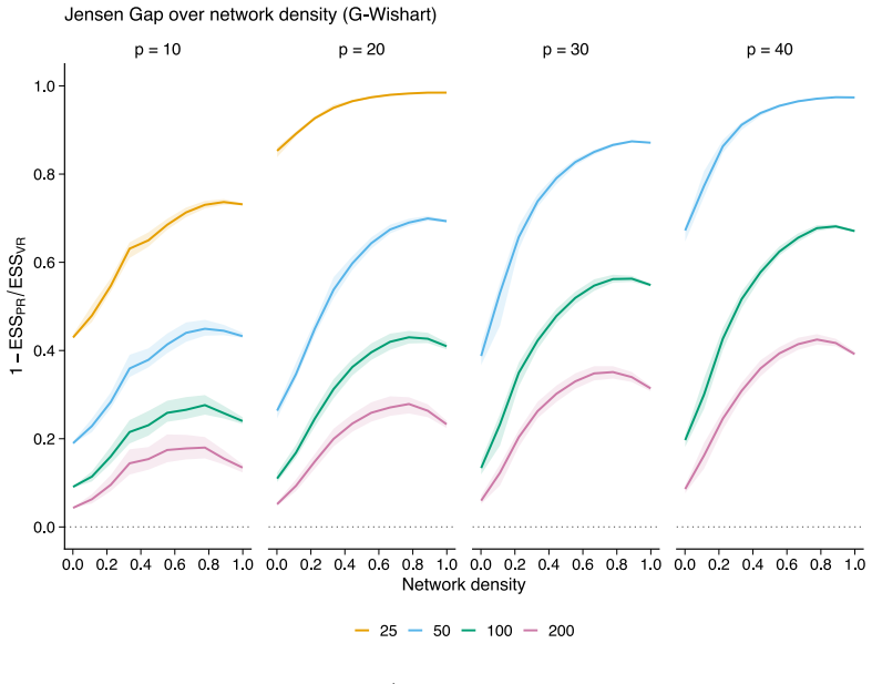
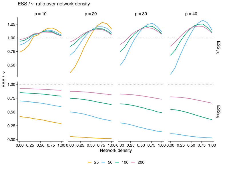
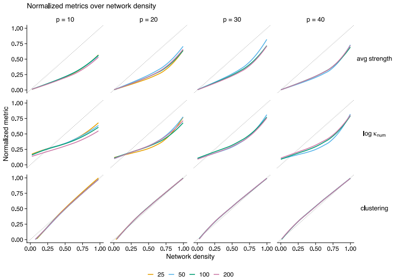
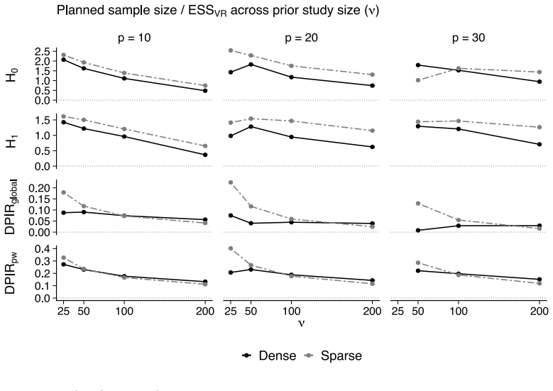
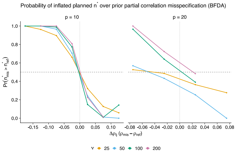
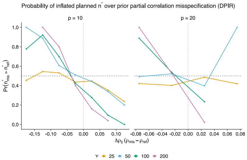
The authors formalize a pre-data effective sample size for GGMs under the Wishart and G-Wishart priors. They adapt five ESS estimators and compute each through a global determinant-ratio scheme and a parameterwise Cholesky scheme. These measures then underpin a Data-to-Prior Information Ratio that identifies when data dominate the prior and a GGM version of Bayes Factor Design Analysis that identifies the sample size needed for conclusive edge evidence. Simulations show the two procedures address complementary design goals and that the estimators respond differently to network structure.
What carries the argument
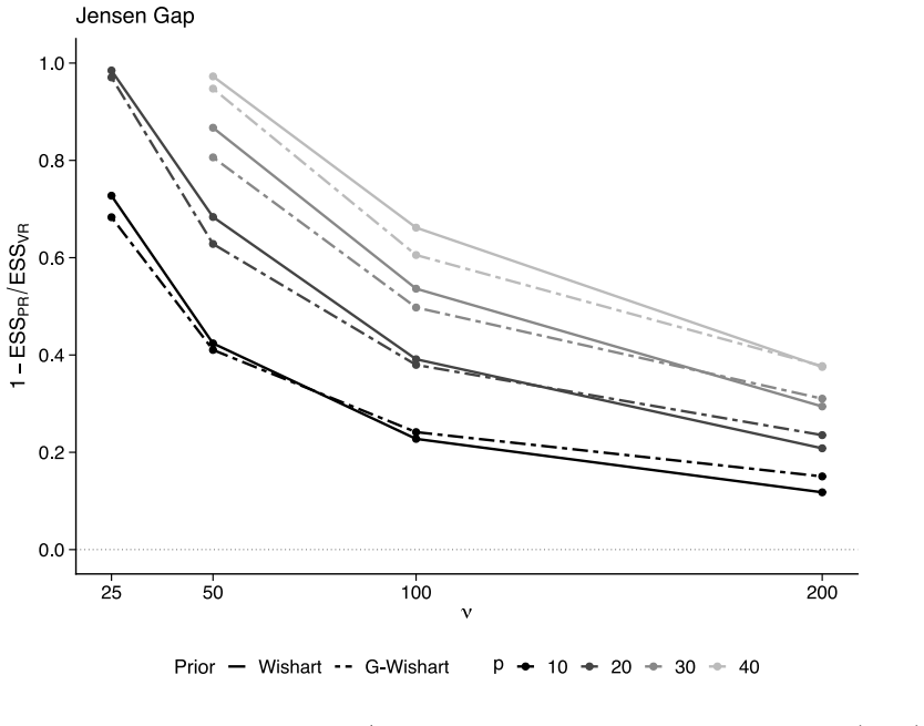
Pre-data effective sample size (ESS) for GGMs, obtained by adapting five estimators and aggregating them globally by determinant ratio or parameterwise by Cholesky decomposition.
If this is right
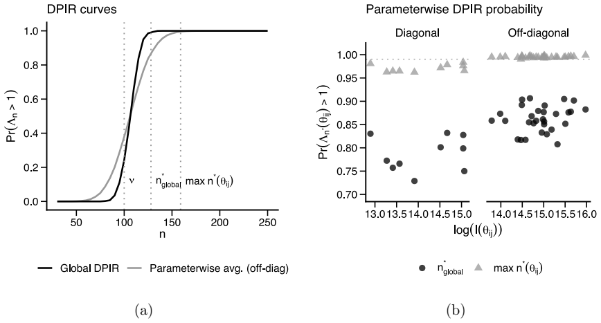
- The Data-to-Prior Information Ratio identifies the smallest sample size at which the data dominate the prior.
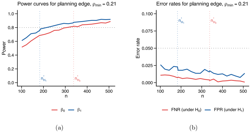
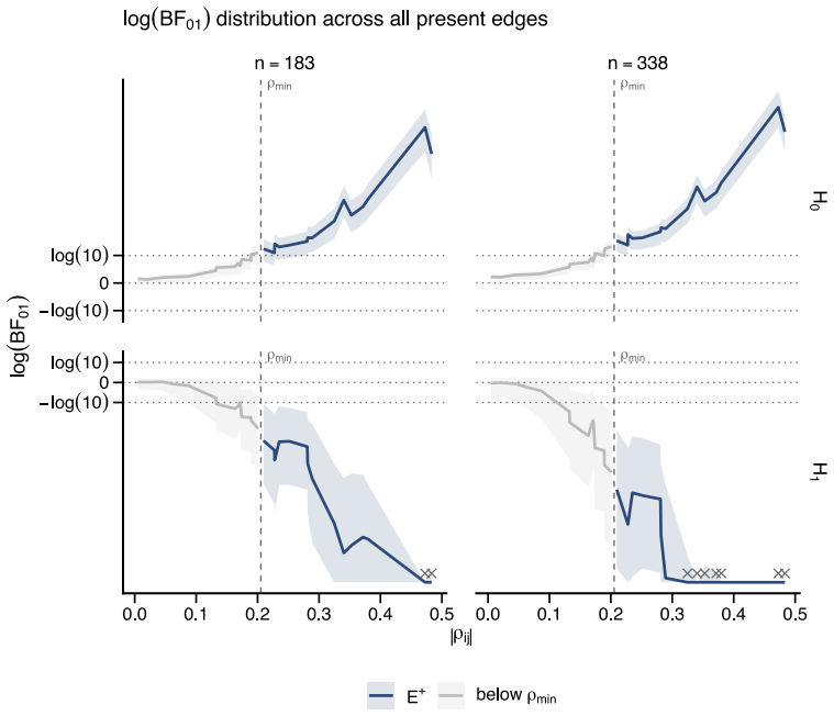
- The extended Bayes Factor Design Analysis identifies the sample size required for conclusive edge-based Bayes factor evidence.
- Different ESS estimators produce systematically different planning recommendations because they vary in sensitivity to network structure and geometry.
- The same machinery applies equally to the Wishart and the G-Wishart prior.
Where Pith is reading between the lines
- The measures could be checked against actual posterior concentration in small-sample real-data analyses to see whether the predicted dominance occurs at the planned sizes.
- Applying the same aggregation logic to other matrix-variate priors might reveal whether the dependence structure of GGMs is unusually difficult to express in observation units.
- Comparing the resulting ESS values across different graphical-model families could show whether the planning tools transfer without modification.
Load-bearing premise
The five ESS estimators remain valid after adaptation to the dependence among precision-matrix entries induced by the Wishart and G-Wishart priors.
What would settle it
A simulation in which the posterior precision matrix after a sample size equal to the computed ESS does not exhibit the degree of concentration predicted by that ESS value.
Figures
read the original abstract
In Bayesian analysis, the prior effective sample size (ESS) expresses the information carried by a prior distribution in units of observations, quantifying how much independent information the prospective data must provide to outweigh an informative prior elicited from a previous study. For network models such as Gaussian graphical models (GGMs), the prior ESS is not straightforward to compute. The Wishart and G-Wishart priors induce dependence among the entries of the precision matrix, and their informativeness has never been expressed in an interpretable, observation-equivalent unit. As a result, researchers eliciting an informative prior for a GGM have had no principled basis for sample size planning. In this paper, we close this gap by formalizing a pre-data ESS for GGMs under the Wishart and G-Wishart priors. We adapt five ESS estimators to the GGM setting and compute each through two aggregation schemes: a global ESS measure based on a determinant ratio, and a parameterwise version based on a Cholesky decomposition. Building on these measures, we introduce two complementary planning strategies: the Data-to-Prior Information Ratio (DPIR), which determines the sample size at which the data dominate the prior, and a GGM extension of Bayes Factor Design Analysis (BFDA), which determines the sample size required for conclusive edge-based evidence. Simulation studies show that the two procedures target complementary design goals and that the ESS estimators differ systematically in their sensitivity to network structure and geometry. We conclude by outlining extensions to other graphical models, including time-dependent variants, as well as to matrix-variate mixture priors.
Editorial analysis
A structured set of objections, weighed in public.
Referee Report
Summary. The paper formalizes a pre-data effective sample size (ESS) for Gaussian graphical models (GGMs) under Wishart and G-Wishart priors. It adapts five standard ESS estimators from the non-graphical literature, computes each via a global aggregation (determinant ratio) and a parameterwise aggregation (Cholesky decomposition), and uses the resulting measures to define the Data-to-Prior Information Ratio (DPIR) for determining when data dominate the prior and a GGM extension of Bayes Factor Design Analysis (BFDA) for edge-based evidence. Simulation studies are reported to show that the procedures target complementary goals and that the ESS estimators differ in sensitivity to network structure.
Significance. If the adapted ESS quantities correctly map prior degrees of freedom to observation-equivalent units while respecting the conditional-independence constraints of the graph, the work would close a genuine methodological gap and supply concrete, interpretable tools for prior elicitation and sample-size planning in network models. The dual aggregation schemes and the complementary DPIR/BFDA planning rules are potentially useful distinctions.
major comments (3)
- [Section describing adaptation of the five ESS estimators] The manuscript provides no verification that any of the five adapted ESS estimators recover the known ESS values for the complete-graph case (ordinary Wishart prior). Without this check, it is unclear whether the adaptation preserves the observation-equivalent interpretation once the precision matrix is restricted to a graph.
- [Section on parameterwise aggregation via Cholesky decomposition] The parameterwise (Cholesky) aggregation scheme is not shown to be invariant to vertex relabeling. Because the Cholesky factor depends on ordering and the graph induces conditional dependencies, different labelings could produce different ESS values, undermining the claim that the measure quantifies prior informativeness in stable observation units.
- [Section introducing DPIR and BFDA] No analytic or numerical argument is given that the global (determinant-ratio) aggregation remains consistent with the parameterwise scheme when the graph is sparse; if the two schemes diverge systematically under conditional independence constraints, the subsequent DPIR and BFDA rules rest on an ambiguous definition of prior strength.
minor comments (2)
- The abstract states that simulations illustrate sensitivity to network structure and geometry, but the main text should include a table or figure that directly compares the five estimators across the same set of graphs and sample sizes.
- Notation for the two aggregation schemes should be introduced with explicit formulas (e.g., the determinant ratio and the Cholesky-based sum) before they are used in the DPIR and BFDA definitions.
Simulated Author's Rebuttal
Thank you for the detailed and constructive referee report. We address each major comment below, indicating planned revisions where appropriate.
read point-by-point responses
-
Referee: [Section describing adaptation of the five ESS estimators] The manuscript provides no verification that any of the five adapted ESS estimators recover the known ESS values for the complete-graph case (ordinary Wishart prior). Without this check, it is unclear whether the adaptation preserves the observation-equivalent interpretation once the precision matrix is restricted to a graph.
Authors: We agree that explicit verification for the complete-graph (unrestricted Wishart) case is necessary to confirm that the adaptation preserves the standard interpretation. In the revised manuscript we will add a dedicated verification subsection (or appendix) demonstrating recovery of the known ESS values under the ordinary Wishart prior when the graph is complete. revision: yes
-
Referee: [Section on parameterwise aggregation via Cholesky decomposition] The parameterwise (Cholesky) aggregation scheme is not shown to be invariant to vertex relabeling. Because the Cholesky factor depends on ordering and the graph induces conditional dependencies, different labelings could produce different ESS values, undermining the claim that the measure quantifies prior informativeness in stable observation units.
Authors: This is a substantive point. The Cholesky factor is ordering-dependent. In revision we will (i) explicitly state that the parameterwise ESS is defined with respect to a fixed, user-chosen vertex ordering consistent with the supplied graph, (ii) add numerical checks across random relabelings in the simulation studies, and (iii) discuss practical recommendations for choosing or stabilizing the ordering. revision: partial
-
Referee: [Section introducing DPIR and BFDA] No analytic or numerical argument is given that the global (determinant-ratio) aggregation remains consistent with the parameterwise scheme when the graph is sparse; if the two schemes diverge systematically under conditional independence constraints, the subsequent DPIR and BFDA rules rest on an ambiguous definition of prior strength.
Authors: We will strengthen this section by adding targeted numerical comparisons of the two aggregation schemes on sparse graphs within the existing simulation framework. These comparisons will quantify agreement/divergence under conditional independence and will be used to clarify the conditions under which DPIR and BFDA remain well-defined. revision: yes
Circularity Check
No significant circularity detected
full rationale
The paper adapts five existing ESS estimators from the non-graphical literature to the Wishart and G-Wishart priors on GGMs, then applies determinant-ratio and Cholesky aggregation schemes to produce observation-equivalent units. No equations or definitions in the provided abstract or description reduce the new ESS quantities to fitted parameters or to the target result by construction. The central formalization is presented as an extension of independent prior work, with simulation studies offered as external checks. This meets the criteria for a self-contained derivation against external benchmarks.
Axiom & Free-Parameter Ledger
Reference graph
Works this paper leans on
-
[1]
Fisher, R. A. , year =. Frequency Distribution of the Values of the Correlation Coefficient in Samples from an Indefinitely Large Population , volume =. Biometrika , publisher =. doi:10.2307/2331838 , number =
-
[2]
On random graph , volume =
Renyi, Erdos , journal =. On random graph , volume =
-
[3]
, title =
Jeffreys, H. , title =. 1961 , edition =
1961
-
[4]
The Annals of Mathematical Statistics , author =
Dickey, James M. , year =. The Weighted Likelihood Ratio, Linear Hypotheses on Normal Location Parameters , volume =. The Annals of Mathematical Statistics , publisher =. doi:10.1214/aoms/1177693507 , number =
-
[5]
, journal =
Dempster, A.P. , journal =. Covariance selection , volume =
-
[6]
Statistical Power Analysis for the Behavioral Sciences , ISBN =
Cohen, Jacob , year =. Statistical Power Analysis for the Behavioral Sciences , ISBN =. doi:10.4324/9780203771587 , publisher =
-
[7]
Dawid, A. P. and Lauritzen, S. L. , year =. Hyper Markov Laws in the Statistical Analysis of Decomposable Graphical Models , volume =. The Annals of Statistics , publisher =. doi:10.1214/aos/1176349260 , number =
-
[8]
, publisher =
Lauritzen, Steffen L. , publisher =. Graphical Models , year =
-
[9]
Bhatia, Rajendra , year =. Matrix Analysis , ISBN =. doi:10.1007/978-1-4612-0653-8 , journal =
-
[10]
Clarke, Bertrand , year =. Implications of Reference Priors for Prior Information and for Sample Size , volume =. Journal of the American Statistical Association , publisher =. doi:10.1080/01621459.1996.10476674 , number =
-
[11]
and Strogatz, Steven H
Watts, Duncan J. and Strogatz, Steven H. , journal =. Collective dynamics of ‘small-world’ networks , volume =. 1998 , doi =
1998
-
[12]
Statistical mechanics of complex networks,
Albert, Réka and Barabási, Albert-László , year =. Statistical mechanics of complex networks , volume =. Reviews of Modern Physics , publisher =. doi:10.1103/revmodphys.74.47 , number =
-
[13]
Journal of Biopharmaceutical Statistics , volume =
Gene Pennello and Laura Thompson , title =. Journal of Biopharmaceutical Statistics , volume =. 2007 , publisher =. doi:10.1080/10543400701668274 , URL =
-
[14]
Morita, Satoshi and Thall, Peter F. and M\". Determining the Effective Sample Size of a Parametric Prior , volume =. Biometrics , publisher =. 2008 , month = jun, pages =. doi:10.1111/j.1541-0420.2007.00888.x , number =
-
[15]
Humphries, Mark D. and Gurney, Kevin , editor =. Network ‘Small-World-Ness’: A Quantitative Method for Determining Canonical Network Equivalence , volume =. PLoS ONE , publisher =. 2008 , month = apr, pages =. doi:10.1371/journal.pone.0002051 , number =
-
[16]
Hastie, Trevor and Tibshirani, Robert and Friedman, Jerome , year =. The Elements of Statistical Learning , ISBN =. doi:10.1007/978-0-387-84858-7 , journal =
-
[17]
Kr\". Regularized estimation of large-scale gene association networks using graphical Gaussian models , volume =. BMC Bioinformatics , publisher =. doi:10.1186/1471-2105-10-384 , number =
-
[18]
Scott, James G. and Berger, James O. , year =. Bayes and empirical-Bayes multiplicity adjustment in the variable-selection problem , volume =. The Annals of Statistics , publisher =. doi:10.1214/10-aos792 , number =
-
[19]
Borsboom, Denny and Cramer, Angélique O.J. , year =. Network Analysis: An Integrative Approach to the Structure of Psychopathology , volume =. Annual Review of Clinical Psychology , publisher =. doi:10.1146/annurev-clinpsy-050212-185608 , number =
-
[20]
Giulio Costantini and Sacha Epskamp and Denny Borsboom and Marco Perugini and René Mõttus and Lourens J. Waldorp and Angélique O.J. Cramer , keywords =. State of the aRt personality research: A tutorial on network analysis of personality data in R , journal =. 2015 , note =. doi:https://doi.org/10.1016/j.jrp.2014.07.003 , url =
-
[21]
Predictively consistent prior effective sample sizes , volume =
Neuenschwander, Beat and Weber, Sebastian and Schmidli, Heinz and O’Hagan, Anthony , year =. Predictively consistent prior effective sample sizes , volume =. Biometrics , publisher =. doi:10.1111/biom.13252 , number =
-
[22]
Isvoranu, Adela-Maria and Epskamp, Sacha and Waldorp, Lourens J. and Borsboom, Denny , year =. Network Psychometrics with R: A Guide for Behavioral and Social Scientists , ISBN =. doi:10.4324/9781003111238 , publisher =
-
[23]
Bayes factors for zero partial covariances , volume =
Giudici, Paolo , year =. Bayes factors for zero partial covariances , volume =. Journal of Statistical Planning and Inference , publisher =. doi:10.1016/0378-3758(94)00101-z , number =
-
[24]
On Moments of the Inverted Wishart Distribution , volume =
Von Rosen, Dietrich , year =. On Moments of the Inverted Wishart Distribution , volume =. Statistics , publisher =. doi:10.1080/02331889708802613 , number =
-
[25]
Bayesian model selection using encompassing priors , volume =
Klugkist, Irene and Kato, Bernet and Hoijtink, Herbert , year =. Bayesian model selection using encompassing priors , volume =. Statistica Neerlandica , publisher =. doi:10.1111/j.1467-9574.2005.00279.x , number =
-
[26]
Clarke, B. and Yuan, Ao , year =. Closed form expressions for Bayesian sample size , volume =. The Annals of Statistics , publisher =. doi:10.1214/009053606000000308 , number =
-
[27]
Morita, Satoshi and Thall, Peter F. and M\". Evaluating the Impact of Prior Assumptions in Bayesian Biostatistics , volume =. Statistics in Biosciences , publisher =. 2010 , month = mar, pages =. doi:10.1007/s12561-010-9018-x , number =
-
[28]
and Wagenmakers, Eric-Jan , year =
Wetzels, Ruud and Grasman, Raoul P.P.P. and Wagenmakers, Eric-Jan , year =. An encompassing prior generalization of the Savage–Dickey density ratio , volume =. Computational Statistics & Data Analysis , publisher =. doi:10.1016/j.csda.2010.03.016 , number =
-
[29]
Mohammadi, A. and Wit, E. C. , year =. Bayesian Structure Learning in Sparse Gaussian Graphical Models , volume =. Bayesian Analysis , publisher =. doi:10.1214/14-ba889 , number =
-
[30]
Bayes factor design analysis: Planning for compelling evidence , volume =
Sch\". Bayes factor design analysis: Planning for compelling evidence , volume =. Psychonomic Bulletin & Review , publisher =. 2017 , month = mar, pages =. doi:10.3758/s13423-017-1230-y , number =
-
[31]
Stefan, Angelika M. and Gronau, Quentin F. and Sch\". A tutorial on Bayes Factor Design Analysis using an informed prior , volume =. Behavior Research Methods , publisher =. 2019 , month = feb, pages =. doi:10.3758/s13428-018-01189-8 , number =
-
[32]
The Matrix-F Prior for Estimating and Testing Covariance Matrices , volume =
Mulder, Joris and Pericchi, Luis Raúl , year =. The Matrix-F Prior for Estimating and Testing Covariance Matrices , volume =. Bayesian Analysis , publisher =. doi:10.1214/17-ba1092 , number =
-
[33]
Mohammadi, Reza and Wit, Ernst C. , year =. BDgraph: An R Package for Bayesian Structure Learning in Graphical Models , volume =. Journal of Statistical Software , publisher =. doi:10.18637/jss.v089.i03 , number =
-
[34]
Vats, Dootika and Flegal, James M and Jones, Galin L , year =. Multivariate output analysis for Markov chain Monte Carlo , volume =. Biometrika , publisher =. doi:10.1093/biomet/asz002 , number =
-
[35]
Quantification of prior impact in terms of effective current sample size , volume =
Wiesenfarth, Manuel and Calderazzo, Silvia , year =. Quantification of prior impact in terms of effective current sample size , volume =. Biometrics , publisher =. doi:10.1111/biom.13124 , number =
-
[36]
BGGM: Bayesian Gaussian Graphical Models in R , volume =
Williams, Donald and Mulder, Joris , year =. BGGM: Bayesian Gaussian Graphical Models in R , volume =. Journal of Open Source Software , publisher =. doi:10.21105/joss.02111 , number =
-
[37]
Astroparticle Physics , keywords =
Williams, Donald R. and Mulder, Joris , year =. Bayesian hypothesis testing for Gaussian graphical models: Conditional independence and order constraints , volume =. doi:10.1016/j.jmp.2020.102441 , journal =
-
[38]
Mulder, Joris and Wagenmakers, Eric-Jan and Marsman, Maarten , year =. A Generalization of the Savage–Dickey Density Ratio for Testing Equality and Order Constrained Hypotheses , volume =. The American Statistician , publisher =. doi:10.1080/00031305.2020.1799861 , number =
work page internal anchor Pith review Pith/arXiv arXiv doi:10.1080/00031305.2020.1799861 2020
-
[39]
Reimherr, Matthew and Meng, Xiao-Li and Nicolae, Dan L. , year =. Prior Sample Size Extensions for Assessing Prior Impact and Prior-Likelihood Discordance , volume =. Journal of the Royal Statistical Society Series B: Statistical Methodology , publisher =. doi:10.1111/rssb.12414 , number =
-
[40]
Jones, David E. and Trangucci, Robert N. and Chen, Yang , year =. Quantifying Observed Prior Impact , volume =. Bayesian Analysis , publisher =. doi:10.1214/21-ba1271 , number =
-
[41]
2019 , eprint=
An empirical G -Wishart prior for sparse high-dimensional Gaussian graphical models , author=. 2019 , eprint=
2019
-
[42]
A Monte Carlo Method for Computing the Marginal Likelihood in Nondecomposable Gaussian Graphical Models , urldate =
Aliye Atay-Kayis and Hélène Massam , journal =. A Monte Carlo Method for Computing the Marginal Likelihood in Nondecomposable Gaussian Graphical Models , urldate =
-
[43]
Cholesky decomposition of a hyper inverse Wishart matrix , volume =
Roverato, A , year =. Cholesky decomposition of a hyper inverse Wishart matrix , volume =. Biometrika , publisher =. doi:10.1093/biomet/87.1.99 , number =
-
[44]
Roverato, Alberto , year =. Hyper Inverse Wishart Distribution for Non‐decomposable Graphs and its Application to Bayesian Inference for Gaussian Graphical Models , volume =. Scandinavian Journal of Statistics , publisher =. doi:10.1111/1467-9469.00297 , number =
-
[45]
A direct sampler for G‐Wishart variates , volume =
Lenkoski, Alex , year =. A direct sampler for G‐Wishart variates , volume =. Stat , publisher =. doi:10.1002/sta4.23 , number =
-
[46]
Magnus and H
J.R. Magnus and H. Neudecker. The elimination matrix: Some lemmas and applications. SIAM Journal on Algebraic and Discrete Methods. 1980
1980
-
[47]
Expected Value of Matrix Quadratic Forms with Wishart distributed Random Matrices , publisher =
Hagedorn, Melinda , keywords =. Expected Value of Matrix Quadratic Forms with Wishart distributed Random Matrices , publisher =. 2022 , copyright =. doi:10.48550/ARXIV.2212.01412 , url =
-
[48]
Marsman, Maarten and van den Bergh, Don and Haslbeck, Jonas M. B. , year =. Bayesian Analysis of the Ordinal Markov Random Field , volume =. Psychometrika , publisher =. doi:10.1017/psy.2024.4 , number =
-
[49]
Arena, Giuseppe , year =
-
[50]
Wild, Beate and Eichler, Michael and Friederich, Hans-Christoph and Hartmann, Mechthild and Zipfel, Stephan and Herzog, Wolfgang , year =. A graphical vector autoregressive modelling approach to the analysis of electronic diary data , volume =. BMC Medical Research Methodology , publisher =. doi:10.1186/1471-2288-10-28 , number =
-
[51]
and Mõttus, René and Borsboom, Denny , year =
Epskamp, Sacha and Waldorp, Lourens J. and Mõttus, René and Borsboom, Denny , year =. The Gaussian Graphical Model in Cross-Sectional and Time-Series Data , volume =. Multivariate Behavioral Research , publisher =. doi:10.1080/00273171.2018.1454823 , number =
-
[52]
and Barabási, A.-L
Albert, R. and Barabási, A.-L. (2002). Statistical mechanics of complex networks. Reviews of Modern Physics , 74(1):47–97
2002
-
[53]
Arena, G. (2026). designbgm : Sample size planning and effective sample size for Bayesian graphical models . R package version 0.1.0
2026
-
[54]
and Massam, H
Atay-Kayis, A. and Massam, H. (2005). A monte carlo method for computing the marginal likelihood in nondecomposable gaussian graphical models. Biometrika , 92(2):317--335
2005
-
[55]
Bhatia, R. (1997). Matrix Analysis . Springer New York
1997
-
[56]
and Cramer, A
Borsboom, D. and Cramer, A. O. (2013). Network analysis: An integrative approach to the structure of psychopathology. Annual Review of Clinical Psychology , 9(1):91–121
2013
-
[57]
Clarke, B. (1996). Implications of reference priors for prior information and for sample size. Journal of the American Statistical Association , 91(433):173–184
1996
-
[58]
and Yuan, A
Clarke, B. and Yuan, A. (2006). Closed form expressions for bayesian sample size. The Annals of Statistics , 34(3)
2006
-
[59]
Cohen, J. (1988). Statistical Power Analysis for the Behavioral Sciences . Routledge
1988
-
[60]
J., and Cramer, A
Costantini, G., Epskamp, S., Borsboom, D., Perugini, M., Mõttus, R., Waldorp, L. J., and Cramer, A. O. (2015). State of the art personality research: A tutorial on network analysis of personality data in r. Journal of Research in Personality , 54:13--29. R Special Issue
2015
-
[61]
Dawid, A. P. and Lauritzen, S. L. (1993). Hyper markov laws in the statistical analysis of decomposable graphical models. The Annals of Statistics , 21(3)
1993
-
[62]
Dempster, A. (1972). Covariance selection. Biometrics , 28:157--175
1972
-
[63]
Dickey, J. M. (1971). The weighted likelihood ratio, linear hypotheses on normal location parameters. The Annals of Mathematical Statistics , 42(1):204–223
1971
-
[64]
J., Mõttus, R., and Borsboom, D
Epskamp, S., Waldorp, L. J., Mõttus, R., and Borsboom, D. (2018). The gaussian graphical model in cross-sectional and time-series data. Multivariate Behavioral Research , 53(4):453–480
2018
-
[65]
Fisher, R. A. (1915). Frequency distribution of the values of the correlation coefficient in samples from an indefinitely large population. Biometrika , 10(4):507
1915
-
[66]
Giudici, P. (1995). Bayes factors for zero partial covariances. Journal of Statistical Planning and Inference , 46(2):161–174
1995
-
[67]
Hagedorn, M. (2022). Expected value of matrix quadratic forms with wishart distributed random matrices
2022
-
[68]
Hastie, T., Tibshirani, R., and Friedman, J. (2009). The Elements of Statistical Learning . Springer New York
2009
-
[69]
Humphries, M. D. and Gurney, K. (2008). Network ‘small-world-ness’: A quantitative method for determining canonical network equivalence. PLoS ONE , 3(4):e0002051
2008
-
[70]
J., and Borsboom, D
Isvoranu, A.-M., Epskamp, S., Waldorp, L. J., and Borsboom, D. (2022). Network Psychometrics with R: A Guide for Behavioral and Social Scientists . Routledge
2022
-
[71]
Jeffreys, H. (1961). Theory of probability . Oxford University Press, Oxford, England, third edition
1961
-
[72]
E., Trangucci, R
Jones, D. E., Trangucci, R. N., and Chen, Y. (2022). Quantifying observed prior impact. Bayesian Analysis , 17(3)
2022
-
[73]
Klugkist, I., Kato, B., and Hoijtink, H. (2005). Bayesian model selection using encompassing priors. Statistica Neerlandica , 59(1):57–69
2005
-
[74]
a mer, N., Sch\
Kr\" a mer, N., Sch\" a fer, J., and Boulesteix, A.-L. (2009). Regularized estimation of large-scale gene association networks using graphical gaussian models. BMC Bioinformatics , 10(1)
2009
-
[75]
Lauritzen, S. L. (1996). Graphical Models . Oxford University Press
1996
-
[76]
Lenkoski, A. (2013). A direct sampler for g‐wishart variates. Stat , 2(1):119–128
2013
-
[77]
and Neudecker, H
Magnus, J. and Neudecker, H. (1980). The elimination matrix: Some lemmas and applications. SIAM Journal on Algebraic and Discrete Methods , 1(4):422--449. Pagination: 28
1980
-
[78]
Marsman, M., van den Bergh, D., and Haslbeck, J. M. B. (2025). Bayesian analysis of the ordinal markov random field. Psychometrika , 90(1):146–182
2025
-
[79]
and Wit, E
Mohammadi, A. and Wit, E. C. (2015). Bayesian structure learning in sparse gaussian graphical models. Bayesian Analysis , 10(1)
2015
-
[80]
and Wit, E
Mohammadi, R. and Wit, E. C. (2019). Bdgraph: An r package for bayesian structure learning in graphical models. Journal of Statistical Software , 89(3)
2019
discussion (0)
Sign in with ORCID, Apple, or X to comment. Anyone can read and Pith papers without signing in.