REVIEW 4 major objections 4 minor 61 references
Dense gas tracers in and between spiral arms: from Giant Molecular Filaments to star-forming clumps
T0 review · 4 major / 4 minor · reviewed 2026-08-07 · deepseek-v4-flash
Pith's one-line read Across two giant molecular filaments, N2H+ emission is uniform between a spiral arm and an interarm region, while CO, HCN, and HCO+ brighten in the arm, implying dense-gas ratio differences are set by moderate-density gas.
desk verdict Valuable new maps and a thorough statistical analysis of dense gas tracers, but the central arm-interarm comparison is probably confounded by a factor-of-1.55 distance mismatch that is never corrected for in the analysis. read the letter →
The pith
A machine-rendered reading of the paper's core claim, the machinery that carries it, and where it could break.
The reading
What carries the argument
The central machinery is a multi-tracer, multi-scale comparison built on 30-m single-dish maps of HCN(1−0), HCO+(1−0), and N2H+(1−0) together with the COHRS 12CO(3−2), CHIMPS 13CO(3−2), and PPMAP N(H2)dust maps. Filling factors, cumulative emission fractions, characteristic column densities N(H2)char, line-to-mass ratios h_Q, and six integrated-intensity ratios are computed per observing region, per filament, and inside dendrogram-defined N2H+ clumps; two-sample Kolmogorov–Smirnov tests compare arm versus interarm and filament versus clump distributions. The load-bearing identity is that N2H+ behaves unlike the other tracers: its emission is concentrated in a tiny fraction of the area, appears only above high column density, and is uniform across environments, while 13CO, HCN, and HCO+ respond to the arm/interarm difference.
What would settle it
Observe the same five tracers toward a distance- and mass-matched sample of several Sagittarius-arm and interarm GMFs; the claim predicts N2H+ integrated-intensity distributions remain statistically indistinguishable (as in the KS test p=0.39 here) while 13CO, HCN, and HCO+ distributions shift brighter in the arm. If N2H+ turns out to brighten or change filling factor systematically with environment in that sample, the uniform-N2H+ claim is falsified.
Extended reading notes
Core claim
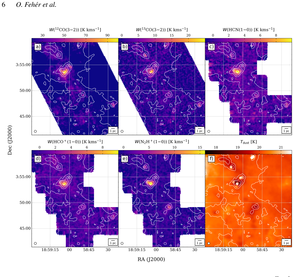
On the two GMFs studied here, N2H+(1−0) is the best tracer of truly dense gas: it has the lowest global filling factor (1.5% in the arm, 7.1% in the interarm), yet its cumulative emission rises latest with column density and its characteristic column density N(H2)char is the highest among the five species (2.4×$10^{22}$ $cm^{-2}$ in the arm, 1.5×$10^{22}$ $cm^{-2}$ in the interarm). While 13CO(3−2), HCN(1−0), and HCO+(1−0) are significantly brighter in the arm filament than in the interarm filament, N2H+ emission is statistically consistent between the two environments (KS test p = 0.39 on filament scale). The arm–interarm differences in the N2H+/13CO and N2H+/HCN ratios therefore come from the 13CO and HCN denominators, not from N2H+. Inside the N2H+-clumps, HCO+ is the only tracer whose emission distribution differs between the two environments; the clumps show the same line-ratio distributions. A consequence is that estimating the global star formation rate of these GMFs from Hi-GAL dust clumps yields more than four times the rate obtained when only N2H+-traced structures are used, even though the arm still contributes about 65% of the total in either case.
Load-bearing premise
The arm-versus-interarm conclusions rest on two filaments, one per environment; if these particular clouds are not representative of their environment, the uniform N2H+ result and the brightening of the other tracers could be coincidences of cloud identity rather than environment.
Editorial extensions
If this is right
- In extragalactic observations, an unresolved increase in N2H+/HCN or N2H+/13CO should be read as a change in the moderate-density gas (CO, HCN, HCO+) rather than as a change in the dense, star-forming gas.
- Star formation rates estimated from dust-based clump catalogs alone may overestimate the true rate by more than a factor of four relative to N2H+-based estimates.
- Observed line-ratio variation within a single filament can be larger than the arm–interarm difference, so single-beam ratio measurements are poor environment indicators.
- The uniformity of N2H+ between arm and interarm supports the view that once dense clumps form, their internal properties become largely independent of the large-scale environment.
Reading between the lines
- The paper's two-cloud sample cannot separate environment from cloud identity; a natural testable extension is to map the same tracer set over a distance-matched sample of several arm and interarm GMFs, predicting N2H+ filling factor and brightness remain low and uniform while HCN and 13CO follow the arm.
- The arm's lower clump fraction (2.8% versus 7.0% at the 3σ boundary) might partly reflect beam dilution of the more distant interarm filament; the authors note the interarm cloud is more distant, and the larger apparent clump sizes there are consistent with this bias.
- The near-constant HCO+/HCN ratio across environments, alongside individually varying HCN and HCO+, suggests these two molecules respond to the same moderate-density gas and radiation conditions, so their ratio may be a more robust environment-independent scale than either line alone.
Editorial analysis
A structured set of objections, weighed in public.
Referee Report
Summary. The paper presents IRAM 30m maps of HCN(1-0), HCO+(1-0), and N2H+(1-0) toward two Giant Molecular Filaments, one in the Sagittarius spiral arm and one in an interarm region, combined with COHRS 12CO(3-2), CHIMPS 13CO(3-2), and Herschel/PPMAP dust column density maps. The authors compute filling factors, cumulative coverage and cumulative emission fractions as functions of column density, molecular line ratios, line-to-mass ratios, clump-averaged correlations, and two-sample Kolmogorov-Smirnov tests. The central claim is that N2H+ has the lowest filling factor but traces the highest-column-density gas best, that its emission is similar in the arm and the interarm, and that the observed variations in ratios such as N2H+/HCN and N2H+/13CO are driven by the moderate-density tracers 13CO, HCN, and HCO+, not by the dense star-forming gas traced by N2H+.
Significance. If the conclusions hold, this is a useful multi-tracer, multi-scale measurement from parsec-sized clumps to tens-of-parsec filaments, directly relevant to interpreting unresolved extragalactic dense-gas observations. The paper's strengths are its direct, checkable observational quantities; the data availability statement; the use of several independent statistical descriptions (cumulative distributions, box plots, Spearman correlations, KS tests); and the explicit acknowledgment of its own limitations in Sections 4.1.2 and 4.2. The main novelty is the contrast between N2H+ and the other tracers across two environments. However, the environmental interpretation is currently underdetermined by the one-arm/one-interarm sample and by the lack of physical-resolution matching, so the significance as a general statement about environments is not yet established.
major comments (4)
- [Sections 2.3, 3.2, 3.3, 4.2, Table 5] The arm/interarm comparison is made at matched angular resolution but not at matched physical resolution. From the physical areas quoted in Section 4.2 (interarm 13CO 2-sigma contour area 316.6 pc^2 versus arm 132.2 pc^2 over nearly equal angular areas), the interarm GMF appears to be about 1.55 times more distant. The IRAM 27-arcsec and JCMT 15-arcsec beams therefore subtend about 1.55 times larger linear scales in the interarm. Since Table 2 shows filling factors of 1-30%, the emission is clumpy and partially resolved, so beam dilution will act more strongly on the interarm maps. This affects the filling factors, the cumulative fractions in Figs 9-11, the line ratios in Table 3, and the KS tests in Table 5, yet the only mention of beam dilution in Section 4.2 concerns clump sizes. The central claim that 13CO, HCN, and HCO+ are brighter in the arm while N2H+ is similar could be a distance-dependent resolution effect. I ask the authors to either convolve all maps to a common physical resolution, or model the beam-dilution effect quantitatively and show that the conclusions survive, or explicitly restate the conclusions as angular-resolution-dependent statements.
- [Sections 4.1.2, 4.2, Conclusions] The environmental conclusions rest on one spiral-arm GMF and one interarm GMF. The paper itself states in Section 4.1.2 that the data 'does not allow for conclusions as a function of Galactic radius' and in Section 4.2 that 'to speculate on the underlying effects requires more observational examples.' Despite these caveats, the abstract and conclusions (iii) present as general findings that the dense-gas tracer behaviour is similar across environments and that ratio differences are driven by moderate-density gas. I recommend either enlarging the sample, or consistently framing the results as a two-object case study and removing the generalizing statements, so that the limitations stated in the text are reflected in the abstract and conclusions.
- [Section 4.2] The clump fraction comparison is sensitive to partly subjective choices and to the distance difference. The arm values are 1.5% at the 2-sigma 13CO contour and 2.8% at the 3-sigma contour, while the interarm values are 2.6% and 7.0%, so the arm/interarm ratio changes from about 1.7 to 2.5 depending on the contour threshold. In addition, because the interarm GMF is more distant, the same angular clump size corresponds to a larger physical area, and the authors themselves note that beam dilution 'might make the detected clumps appear larger there.' A quantitative demonstration that the arm/interarm difference in clump fraction survives both the contour choice and the distance-dependent resolution is needed before this result can support the star-formation discussion in Section 4.2.
- [Section 3.4 and Table 5] The statistical presentation needs clarification. In Section 3.4 the text reads 'fairly tight correlations (p-value>0.5)'; a p-value above 0.5 would indicate no significant correlation, so this should read 'correlation coefficient > 0.5' or similar. The description of the KS tests in Section 4.1.2 says the data are binned into 30 bins before the tests, which would invalidate the use of ks_2samp on continuous distributions; if the binning is only for the histograms in Figs 16-17, this should be stated explicitly. The caption of Table 5 also misnumbers its columns, referring to repeated '(3)' and four entries while the text refers to the second, third, fourth, and fifth columns.
minor comments (4)
- [Section 2.2/2.3] Please state explicitly that the maps are resampled to a common pixel size but not convolved to a common angular resolution before the point-by-point comparisons, and note the expected effect on ratio maps such as N2H+/13CO where the two transitions have different beam sizes.
- [Section 4.2] The distances to the two GMFs are not given explicitly in this paper; providing them, together with the physical beam sizes at each distance, would make the beam-dilution discussion reproducible without requiring the reader to reconstruct the distances from the quoted physical areas.
- [Table 5] A closing parenthesis is missing in the HCO+ row for the KS2 arm column ('1.3×10⁻⁶' should be '1.3×10⁻⁶)'), and the column headings should be renumbered to match the text.
- [Section 3.1 and Table 1] The velocity integration windows in Table 1 vary by region and by species, especially for HCO+. A short justification of why the windows for HCO+ differ from those of the other species at the same v_LSR would help the reader assess how much of the measured ratio differences could come from the integration choices.
Circularity Check
No significant circularity: the paper's conclusions are direct statistics on observed maps, with no fitted parameter renamed as a prediction and no load-bearing self-citation chain.
full rationale
I find no circular step that meets the bar of Eq X = Eq Y by construction or a fitted parameter renamed as a prediction. The integrated intensities, filling factors, cumulative fractions, characteristic column densities, line ratios, and KS-test results are all direct statistics computed from observed maps (IRAM 30m, CHIMPS, COHRS, and Herschel/PPMAP). The quantity N(H2)char is explicitly defined as the column density below which 50% of a line's emission originates, so stating that N2H+ has the highest N(H2)char is a restatement of the measured cumulative fraction, not a derived physical prediction; this is descriptive quantile reporting, not circular derivation. The N2H+-clump catalog is inherited from the same authors' Fehér et al. (2024), and the paper cites Priestley et al. (2023b) for the chemical reliability of N2H+, but the central arm-versus-interarm comparisons are computed from the newly presented HCN and HCO+ maps together with published CO and dust data; the conclusions do not reduce to accepting those self-citations. The paper also flags its own limitations: Section 4.1.2 states the data 'does not allow for conclusions as a function of Galactic radius,' and Section 4.2 notes 'to speculate on the underlying effects requires more observational examples' and acknowledges that 'beam dilution towards the more distant cloud, the interarm GMF, might make the detected clumps appear larger there.' These caveats weaken generalizability and raise a possible resolution-matching concern, but they are honesty about confounds and sample size, not circularity. The derivation chain is self-contained as observational analysis.
Assumptions & free parameters
free parameters (5)
- 3-sigma detection threshold for filling factors and cumulative fractions =
3 (multiple of sigma_int)
- 2-sigma threshold for molecular ratio maps and averages =
2 (multiple of sigma_int)
- Per-region velocity integration windows =
values in Table 1, e.g., 60-105 km/s for interarm, 31-64 km/s for arm 13CO
- Column density bin percentages for line-to-mass ratio =
[5-10% by 0.5%, 10-30% by 5%, 50, 80, 100% of N(H2)_dust max]
- Clump fraction contour level =
2 sigma_int (2.4 K km/s) and 3 sigma_int of W(13CO)
assumptions (4)
- domain assumption PPMAP dust column density maps accurately trace total H2 column density
- domain assumption N2H+(1-0) emission traces dense star-forming gas
- domain assumption The two GMFs are representative of arm and interarm environments
- domain assumption Elia et al. (2022) SFR formula applies to these clumps
Cite this review
Pith. "Pith review of Dense gas tracers in and between spiral arms: from Giant Molecular Filaments to star-forming clumps." pith.science (2026). https://pith.science/paper/5HICYHEF
@misc{pith2026250524711,
  author       = {Pith},
  title        = {Pith review of: Dense gas tracers in and between spiral arms: from Giant Molecular Filaments to star-forming clumps},
  year         = {2026},
  howpublished = {\url{https://pith.science/paper/5HICYHEF}},
  note         = {Machine review of arXiv:2505.24711}
}
abstract
Giant Molecular Filaments are opportune locations in our Galaxy to study the star-forming interstellar matter and its accumulation on spatial scales comparable to those now becoming available for external galaxies. We mapped the emission of HCN(1$-$0), HCO$^+$(1$-$0), and N$_2$H$^+$(1$-$0) towards two of these filaments, one associated with the Sagittarius arm and one with an interarm area. Using the data alongside the COHRS $^{12}$CO(3$-$2), the CHIMPS $^{13}$CO(3$-$2), and $\textit{Herschel}$-based column density maps, we evaluate the dense gas tracer emission characteristics and find that although its filling factor is the smallest among the studied species, N$_2$H$^+$ is the best at tracing the truly dense gas. Significant differences can be seen between the $^{13}$CO, HCN, and $N$(H$_2$)$_{\mathrm{dust}}$ levels of the arm and interarm, while the N$_2$H$^+$ emission is more uniform regardless of location, meaning that the observed variations in line ratios like N$_2$H$^+$/HCN or N$_2$H$^+$/$^{13}$CO are driven by species tracing moderate-density gas and not the star-forming gas. In many cases, greater variation in molecular emission and ratios exist between regions inside a filament than between the arm and interarm environments. The choice of measure of the dense gas and the available spatial resolution have deep impact on the multi-scale view of different environments inside a galaxy regarding molecular emissions, ratios, and thus the estimated star formation activity.
Figures


Figures from the paper (17 more)



Reference graph
Works this paper leans on
-
[1]
Abreu-Vicente J., Ragan S., Kainulainen J., Henning T., Beuther H., Johnston K., 2016, @doi [ ] 10.1051/0004-6361/201527674 , https://ui.adsabs.harvard.edu/abs/2016A&A...590A.131A 590, A131
-
[2]
Andr \'e P., Di Francesco J., Ward-Thompson D., Inutsuka S. I., Pudritz R. E., Pineda J. E., 2014, @doi [Protostars and Planets VI] 10.2458/azu_uapress_9780816531240-ch002 , https://ui.adsabs.harvard.edu/abs/2014prpl.conf...27A p. 27
-
[3]
Astropy Collaboration et al., 2022, @doi [ ] 10.3847/1538-4357/ac7c74 , https://ui.adsabs.harvard.edu/abs/2022ApJ...935..167A 935, 167
-
[4]
J., Muller E., Indermuehle B., O'Dougherty S
Barnes P. J., Muller E., Indermuehle B., O'Dougherty S. N., Lowe V., Cunningham M., Hernandez A. K., Fuller G. A., 2015, @doi [ ] 10.1088/0004-637X/812/1/6 , https://ui.adsabs.harvard.edu/abs/2015ApJ...812....6B 812, 6
-
[5]
Barnes A. T., et al., 2020, @doi [ ] 10.1093/mnras/staa1814 , https://ui.adsabs.harvard.edu/abs/2020MNRAS.497.1972B 497, 1972
-
[6]
Battisti A. J., Heyer M. H., 2014, @doi [ ] 10.1088/0004-637X/780/2/173 , https://ui.adsabs.harvard.edu/abs/2014ApJ...780..173B 780, 173
-
[7]
Benjamin R. A., et al., 2003, @doi [ ] 10.1086/376696 , https://ui.adsabs.harvard.edu/abs/2003PASP..115..953B 115, 953
doi:10.1086/376696 2003
-
[8]
Bigiel F., Leroy A., Walter F., Brinks E., de Blok W. J. G., Madore B., Thornley M. D., 2008, @doi [ ] 10.1088/0004-6256/136/6/2846 , https://ui.adsabs.harvard.edu/abs/2008AJ....136.2846B 136, 2846
Show all 61 references
-
[9]
C., Glover S
Clark P. C., Glover S. C. O., 2015, @doi [ ] 10.1093/mnras/stv1369 , https://ui.adsabs.harvard.edu/abs/2015MNRAS.452.2057C 452, 2057
2015 doi
-
[10]
Contreras Y., et al., 2013, @doi [ ] 10.1051/0004-6361/201220155 , https://ui.adsabs.harvard.edu/abs/2013A&A...549A..45C 549, A45
2013 doi
-
[11]
T., Thomas H
Dempsey J. T., Thomas H. S., Currie M. J., 2013, @doi [ ] 10.1088/0067-0049/209/1/8 , https://ui.adsabs.harvard.edu/abs/2013ApJS..209....8D 209, 8
2013 doi
-
[12]
J., Moore T
Eden D. J., Moore T. J. T., Morgan L. K., Thompson M. A., Urquhart J. S., 2013, @doi [MNRAS] 10.1093/mnras/stt279 , https://ui.adsabs.harvard.edu/abs/2013MNRAS.431.1587E 431, 1587
2013 doi
-
[13]
Elia D., et al., 2021, @doi [ ] 10.1093/mnras/stab1038 , https://ui.adsabs.harvard.edu/abs/2021MNRAS.504.2742E 504, 2742
2021 doi
-
[14]
Elia D., et al., 2022, @doi [ ] 10.3847/1538-4357/aca27d , https://ui.adsabs.harvard.edu/abs/2022ApJ...941..162E 941, 162
2022 doi
-
[15]
Evans II N. J., Kim K.-T., Wu J., Chao Z., Heyer M., Liu T., Nguyen-Lu'o'ng Q., Kauffmann J., 2020, @doi [ ] 10.3847/1538-4357/ab8938 , https://ui.adsabs.harvard.edu/abs/2020ApJ...894..103E 894, 103
2020 doi
-
[16]
E., Priestley F
Feh \'e r O., Ragan S. E., Priestley F. D., Clark P. C., Moore T. J. T., 2024, @doi [ ] 10.1093/mnras/stae918 , https://ui.adsabs.harvard.edu/abs/2024MNRAS.530.1311F 530, 1311
2024 doi
-
[17]
M., 2004, @doi [ApJ] 10.1086/382999 , https://ui.adsabs.harvard.edu/abs/2004ApJ...606..271G 606, 271
Gao Y., Solomon P. M., 2004, @doi [ApJ] 10.1086/382999 , https://ui.adsabs.harvard.edu/abs/2004ApJ...606..271G 606, 271
2004 doi
-
[18]
E., Heitsch F., Kainulainen J., Panopoulou G
Hacar A., Clark S. E., Heitsch F., Kainulainen J., Panopoulou G. V., Seifried D., Smith R., 2023, in Inutsuka S., Aikawa Y., Muto T., Tomida K., Tamura M., eds, Astronomical Society of the Pacific Conference Series Vol. 534, Protostars and Planets VII. p. 153 ( @eprint arXiv 2...
-
[19]
R., et al., 2020, @doi [Nature] 10.1038/s41586-020-2649-2 , 585, 357
Harris C. R., et al., 2020, @doi [Nature] 10.1038/s41586-020-2649-2 , 585, 357
2020 doi
-
[20]
D., 2007, @doi [Computing in Science & Engineering] 10.1109/MCSE.2007.55 , 9, 90
Hunter J. D., 2007, @doi [Computing in Science & Engineering] 10.1109/MCSE.2007.55 , 9, 90
2007 doi
-
[21]
M., et al., 2006, @doi [ ] 10.1086/500091 , https://ui.adsabs.harvard.edu/abs/2006ApJS..163..145J 163, 145
Jackson J. M., et al., 2006, @doi [ ] 10.1086/500091 , https://ui.adsabs.harvard.edu/abs/2006ApJS..163..145J 163, 145
2006 doi
-
[22]
M., Finn S
Jackson J. M., Finn S. C., Chambers E. T., Rathborne J. M., Simon R., 2010, @doi [ ] 10.1088/2041-8205/719/2/L185 , https://ui.adsabs.harvard.edu/abs/2010ApJ...719L.185J 719, L185
2010 doi
-
[23]
J., et al., 2023, @doi [ ] 10.1051/0004-6361/202347050 , https://ui.adsabs.harvard.edu/abs/2023A&A...676L..11J 676, L11
Jim \'e nez-Donaire M. J., et al., 2023, @doi [ ] 10.1051/0004-6361/202347050 , https://ui.adsabs.harvard.edu/abs/2023A&A...676L..11J 676, L11
2023 doi
-
[24]
H., Clark P
Jones G. H., Clark P. C., Glover S. C. O., Hacar A., 2023, @doi [ ] 10.1093/mnras/stad202 , https://ui.adsabs.harvard.edu/abs/2023MNRAS.520.1005J 520, 1005
2023 doi
-
[25]
A., Mandel E., 2003, in Payne H
Joye W. A., Mandel E., 2003, in Payne H. E., Jedrzejewski R. I., Hook R. N., eds, Astronomical Society of the Pacific Conference Series Vol. 295, Astronomical Data Analysis Software and Systems XII. p. 489
2003
-
[26]
F., Melnick G., Tolls V., Guzman A., Menten K
Kauffmann J., Goldsmith P. F., Melnick G., Tolls V., Guzman A., Menten K. M., 2017, @doi [ ] 10.1051/0004-6361/201731123 , https://ui.adsabs.harvard.edu/abs/2017A&A...605L...5K 605, L5
2017 doi
-
[27]
J., 1998, @doi [ApJ] 10.1086/305588 , https://ui.adsabs.harvard.edu/abs/1998ApJ...498..541K 498, 541
Kennicutt Robert C. J., 1998, @doi [ApJ] 10.1086/305588 , https://ui.adsabs.harvard.edu/abs/1998ApJ...498..541K 498, 541
1998 doi
-
[28]
J., Lombardi M., Alves J
Lada C. J., Lombardi M., Alves J. F., 2010, @doi [ApJ] 10.1088/0004-637X/724/1/687 , https://ui.adsabs.harvard.edu/abs/2010ApJ...724..687L 724, 687
2010 doi
-
[29]
A., Whitworth A
Marsh K. A., Whitworth A. P., Lomax O., 2015, @doi [ ] 10.1093/mnras/stv2248 , https://ui.adsabs.harvard.edu/abs/2015MNRAS.454.4282M 454, 4282
2015 doi
-
[30]
A., et al., 2017, @doi [ ] 10.1093/mnras/stx1723 , https://ui.adsabs.harvard.edu/abs/2017MNRAS.471.2730M 471, 2730
Marsh K. A., et al., 2017, @doi [ ] 10.1093/mnras/stx1723 , https://ui.adsabs.harvard.edu/abs/2017MNRAS.471.2730M 471, 2730
2017 doi
-
[31]
Molinari S., et al., 2010, @doi [ ] 10.1086/651314 , https://ui.adsabs.harvard.edu/abs/2010PASP..122..314M 122, 314
2010 doi
-
[32]
Moore T. J. T., Urquhart J. S., Morgan L. K., Thompson M. A., 2012, @doi [ ] 10.1111/j.1365-2966.2012.21740.x , https://ui.adsabs.harvard.edu/abs/2012MNRAS.426..701M 426, 701
2012
-
[33]
T., Bigiel F., Neumann L., 2023, @doi [ ] 10.1093/mnras/stad1741 , https://ui.adsabs.harvard.edu/abs/2023MNRAS.523.6138P 523, 6138
Panessa M., Seifried D., Walch S., Gaches B., Barnes A. T., Bigiel F., Neumann L., 2023, @doi [ ] 10.1093/mnras/stad1741 , https://ui.adsabs.harvard.edu/abs/2023MNRAS.523.6138P 523, 6138
2023 doi
-
[34]
Park G., et al., 2023, @doi [ ] 10.3847/1538-4365/ac9b59 , https://ui.adsabs.harvard.edu/abs/2023ApJS..264...16P 264, 16
2023 doi
-
[35]
I., Kim K.-T., Heyer M., Kauffmann J., Jose J., Samal M
Patra S., Evans Neal J. I., Kim K.-T., Heyer M., Kauffmann J., Jose J., Samal M. R., Das S. R., 2022, @doi [ ] 10.3847/1538-3881/ac83af , https://ui.adsabs.harvard.edu/abs/2022AJ....164..129P 164, 129
2022 doi
-
[36]
Pety J., et al., 2017, @doi [ ] 10.1051/0004-6361/201629862 , https://ui.adsabs.harvard.edu/abs/2017A&A...599A..98P 599, A98
2017 doi
-
[37]
D., Clark P
Priestley F. D., Clark P. C., Glover S. C. O., Ragan S. E., Feh \'e r O., Prole L. R., Klessen R. S., 2023a, @doi [ ] 10.1093/mnras/stad2278 , https://ui.adsabs.harvard.edu/abs/2023MNRAS.524.5971P 524, 5971
-
[38]
D., Clark P
Priestley F. D., Clark P. C., Glover S. C. O., Ragan S. E., Feh \'e r O., Prole L. R., Klessen R. S., 2023b, @doi [ ] 10.1093/mnras/stad3089 , https://ui.adsabs.harvard.edu/abs/2023MNRAS.526.4952P 526, 4952
-
[39]
D., Clark P
Priestley F. D., Clark P. C., Glover S. C. O., Ragan S. E., Feh \'e r O., Prole L. R., Klessen R. S., 2024, @doi [ ] 10.1093/mnras/stae1442 , https://ui.adsabs.harvard.edu/abs/2024MNRAS.531.4408P 531, 4408
2024 doi
-
[40]
E., Henning T., Tackenberg J., Beuther H., Johnston K
Ragan S. E., Henning T., Tackenberg J., Beuther H., Johnston K. G., Kainulainen J., Linz H., 2014, @doi [ ] 10.1051/0004-6361/201423401 , https://ui.adsabs.harvard.edu/abs/2014A&A...568A..73R 568, A73
2014 doi
-
[41]
E., Moore T
Ragan S. E., Moore T. J. T., Eden D. J., Hoare M. G., Elia D., Molinari S., 2016, @doi [MNRAS] 10.1093/mnras/stw1870 , https://ui.adsabs.harvard.edu/abs/2016MNRAS.462.3123R 462, 3123
2016 doi
-
[42]
J., et al., 2016, @doi [MNRAS] 10.1093/mnras/stv2808 , https://ui.adsabs.harvard.edu/abs/2016MNRAS.456.2885R 456, 2885
Rigby A. J., et al., 2016, @doi [MNRAS] 10.1093/mnras/stv2808 , https://ui.adsabs.harvard.edu/abs/2016MNRAS.456.2885R 456, 2885
2016 doi
- [43]
-
[44]
M., Heyer M., Rathborne J., Simon R., 2010, @doi [ ] 10.1088/0004-637X/723/1/492 , https://ui.adsabs.harvard.edu/abs/2010ApJ...723..492R 723, 492
Roman-Duval J., Jackson J. M., Heyer M., Rathborne J., Simon R., 2010, @doi [ ] 10.1088/0004-637X/723/1/492 , https://ui.adsabs.harvard.edu/abs/2010ApJ...723..492R 723, 492
2010 doi
-
[45]
M., Clark P., Klessen R., Shetty R., 2016, @doi [ ] 10.3847/0004-637X/818/2/144 , https://ui.adsabs.harvard.edu/abs/2016ApJ...818..144R 818, 144
Roman-Duval J., Heyer M., Brunt C. M., Clark P., Klessen R., Shetty R., 2016, @doi [ ] 10.3847/0004-637X/818/2/144 , https://ui.adsabs.harvard.edu/abs/2016ApJ...818..144R 818, 144
2016 doi
-
[46]
K., 2024, @doi [ ] 10.1146/annurev-astro-071221-052651 , https://ui.adsabs.harvard.edu/abs/2024ARA&A..62..369S 62, 369
Schinnerer E., Leroy A. K., 2024, @doi [ ] 10.1146/annurev-astro-071221-052651 , https://ui.adsabs.harvard.edu/abs/2024ARA&A..62..369S 62, 369
2024 doi
-
[47]
Schinnerer E., et al., 2017, @doi [ApJ] 10.3847/1538-4357/836/1/62 , https://ui.adsabs.harvard.edu/abs/2017ApJ...836...62S 836, 62
2017 doi
-
[48]
Schmidt M., 1959, @doi [ApJ] 10.1086/146614 , https://ui.adsabs.harvard.edu/abs/1959ApJ...129..243S 129, 243
1959 doi
-
[49]
C., Klessen R
Shetty R., Clark P. C., Klessen R. S., 2014, @doi [ ] 10.1093/mnras/stu919 , https://ui.adsabs.harvard.edu/abs/2014MNRAS.442.2208S 442, 2208
2014 doi
-
[50]
K., et al., 2023, @doi [ ] 10.1051/0004-6361/202348205 , https://ui.adsabs.harvard.edu/abs/2023A&A...680L..20S 680, L20
Stuber S. K., et al., 2023, @doi [ ] 10.1051/0004-6361/202348205 , https://ui.adsabs.harvard.edu/abs/2023A&A...680L..20S 680, L20
2023 doi
-
[51]
Tafalla M., Usero A., Hacar A., 2021, @doi [ ] 10.1051/0004-6361/202038727 , https://ui.adsabs.harvard.edu/abs/2021A&A...646A..97T 646, A97
2021 doi
-
[52]
Tafalla M., Usero A., Hacar A., 2023, @doi [ ] 10.1051/0004-6361/202346136 , https://ui.adsabs.harvard.edu/abs/2023A&A...679A.112T 679, A112
2023 doi
-
[53]
Veneziani M., et al., 2017, @doi [ ] 10.1051/0004-6361/201423474 , https://ui.adsabs.harvard.edu/abs/2017A&A...599A...7V 599, A7
2017 doi
-
[54]
Virtanen P., et al., 2020, @doi [Nature Methods] 10.1038/s41592-019-0686-2 , https://rdcu.be/b08Wh 17, 261
2020 doi
-
[55]
M., Molinari S., Schisano E., 2015, @doi [ ] 10.1093/mnras/stv735 , https://ui.adsabs.harvard.edu/abs/2015MNRAS.450.4043W 450, 4043
Wang K., Testi L., Ginsburg A., Walmsley C. M., Molinari S., Schisano E., 2015, @doi [ ] 10.1093/mnras/stv735 , https://ui.adsabs.harvard.edu/abs/2015MNRAS.450.4043W 450, 4043
2015 doi
-
[56]
M., Beuther H., Henning T., 2016, @doi [ ] 10.3847/0067-0049/226/1/9 , https://ui.adsabs.harvard.edu/abs/2016ApJS..226....9W 226, 9
Wang K., Testi L., Burkert A., Walmsley C. M., Beuther H., Henning T., 2016, @doi [ ] 10.3847/0067-0049/226/1/9 , https://ui.adsabs.harvard.edu/abs/2016ApJS..226....9W 226, 9
2016 doi
-
[57]
Wang Y., et al., 2020, @doi [ ] 10.1051/0004-6361/202037928 , https://ui.adsabs.harvard.edu/abs/2020A&A...641A..53W 641, A53
2020 doi
-
[58]
I., Shirley Y
Wu J., Evans Neal J. I., Shirley Y. L., Knez C., 2010, @doi [ ] 10.1088/0067-0049/188/2/313 , https://ui.adsabs.harvard.edu/abs/2010ApJS..188..313W 188, 313
2010 doi
-
[59]
Zucker C., Battersby C., Goodman A., 2015, @doi [ApJ] 10.1088/0004-637X/815/1/23 , https://ui.adsabs.harvard.edu/abs/2015ApJ...815...23Z 815, 23
2015 doi
-
[60]
Zucker C., Battersby C., Goodman A., 2018, @doi [ ] 10.3847/1538-4357/aacc66 , https://ui.adsabs.harvard.edu/abs/2018ApJ...864..153Z 864, 153
2018 doi
-
[61]
write newline
" write newline "" before.all 'output.state := FUNCTION fin.entry write newline FUNCTION new.block output.state before.all = 'skip after.block 'output.state := if FUNCTION new.sentence output.state after.block = 'skip output.state before.all = 'skip after.sentence 'output.stat...
Reviewed August 7, 2026 · model on record in the stance chip above.
Discussion (0). Sign in to comment.