Orthogonality Sampling Method for the Electromagnetic Inverse Scattering Problem

Dinh-Liem Nguyen; Isaac Harris

REVIEW 2 major objections 6 minor 20 references

Orthogonality Sampling Method for the Electromagnetic Inverse Scattering Problem

T0 review · 2 major / 6 minor · reviewed 2026-08-14 · deepseek-v4-flash

Challenge this review Re-run · record.json Download PDF Read on arXiv ↗ Review JSON

Pith's one-line read This paper proves that the orthogonality sampling imaging functional—a single inner product of far-field data with a known dipole wave—is positive inside an anisotropic electromagnetic scatterer and decays quadratically outside it…

desk verdict A worthy extension of OSM and DSM to anisotropic electromagnetic scattering, but the decay proof in Theorem 6 has a concrete, load-bearing computational error that must be corrected before the resolution analysis can be trusted. read the letter →

arxiv 1908.05800 v3 pith:5T46OLHP submitted 2019-08-16 math.AP

Isaac Harris , Dinh-Liem Nguyen This is my paper · ORCID

classification math.AP MSC 35R3035R0965R20

keywords orthogonalitysamplingmethoddirectinverseelectromagneticscatteringMaxwell'sequationsanisotropicmediafarfieldoperatorfactorizationFunk-Heckeformula

verification ladder T0 review T1 audit T2 compute T3 formal

The pith

A machine-rendered reading of the paper's core claim, the machinery that carries it, and where it could break.

The reading

The paper establishes a rigorous foundation for the orthogonality sampling method (OSM) in electromagnetic inverse scattering: from fixed-frequency far-field data produced by an anisotropic penetrable scatterer, the imaging functional $I_{\mathrm{OSM}}(y_s)$—computed as a single inner product of the data with a known electric dipole wave—is proved to be bounded below by a positive constant at every sampling point $y_s$ inside the scatterer and to decay like $O(1/\operatorname{dist}(y_s,\Omega)^2)$ outside it. Because this two-sided behaviour holds, plotting the functional over a sampling grid recovers the scatterer's location and shape without solving an ill-posed equation at each point. The paper also proves that the direct sampling method (DSM) functional is equivalent to the OSM functional up to explicit constants, so the DSM inherits the same resolution and decay guarantees, and it proves a stability estimate showing that noise in the far-field data changes the image only to order $\delta$. The result matters because it converts a very cheap imaging heuristic into a quantitative reconstruction tool for three-dimensional anisotropic media, with numerical examples confirming the predicted behaviour.

What carries the argument

The load-bearing object is the factorization of the far-field operator $F=H^*TH$, where $H:L^2_t(S^2)\to L^2(\Omega)^3$ superposes incident plane waves, $H^*$ maps a volume source to its electric dipole far-field pattern, and $T=k^2P(f+v)$ records the contrast-induced source inside the scatterer. Two ingredients make the argument move: the coercivity of $T$ on the range of $H$ (a uniform positivity condition on $\langle Tv,v\rangle$, guaranteed when the contrast $P$ is dissipative in a uniform sense and $k$ is not a transmission eigenvalue) and the range characterization $\varphi_{y_s}\in\operatorname{Range}(H^*)$ if and only if $y_s\in\Omega$. The Funk-Hecke formula, applied to the spherical Bessel function $j_0$, turns these operator facts into the explicit decay rate $O(1/\operatorname{dist}(y_s,\Omega)^2)$ for sampling points outside the scatterer.

What would settle it

Run the OSM on synthetic far-field data for a three-dimensional anisotropic scatterer with a purely real, non-dissipative contrast $P$ at a wave number $k$ that is a transmission eigenvalue, and compare the minimum of $I_{\mathrm{OSM}}$ over the scatterer with its values just outside; if interior values are not bounded away from the exterior background, the coercivity condition in Theorem 4 is exactly what carries the detection property.

Watch

Extended reading notes

Core claim

On the paper's own terms, the central discovery is that the orthogonality sampling functional $I_{\mathrm{OSM}}(y_s)=\|p\cdot F\varphi_{y_s}\|^2_{L^2(S^2)}$ is a reliable indicator of whether a sampling point lies in the scatterer. Theorem 6 proves the two-sided behaviour: for $y_s\in\Omega$ the functional is bounded below by a positive constant, while for $y_s\notin\Omega$ it decays as $O(1/\operatorname{dist}(y_s,\Omega)^2)$ as $y_s$ recedes. The proof runs through the factorization $F=H^*TH$ of the far-field operator into the plane-wave superposition operator $H$, the contrast-dependent middle operator $T=k^2P(f+v)$, and the adjoint $H^*$; when $T$ is coercive on the range of $H$, the functional inherits a positive lower bound exactly on $\Omega$, and the Funk-Hecke formula converts the decay of the spherical Bessel function $j_0$ into the explicit quadratic decay outside. The same ingredients give the equivalence $c_1 I_{\mathrm{OSM}}\le I_{\mathrm{DSM}}\le c_2\sqrt{I_{\mathrm{OSM}}}$, so the direct sampling functional is positive inside and decays like $O(1/\operatorname{dist}(y_s,\Omega)^2)$ outside as well.

Load-bearing premise

The entire inside-scatterer lower bound rests on the contrast $P$ being dissipative enough—either $\operatorname{Im}(P)$ uniformly positive definite, or $\operatorname{Re}(P)+\alpha\operatorname{Im}(P)$ uniformly positive definite with $\operatorname{Im}(P)$ positive semidefinite—and on $k$ not being a transmission eigenvalue; if that material condition fails, the paper does not prove the imaging functional stays positive inside the scatterer.

Editorial extensions

If this is right

Because $I_{\mathrm{OSM}}$ has a uniform positive lower bound on $\Omega$ and decays quadratically outside, thresholding a plot of the functional over a sampling grid yields an estimate of the scatterer's support without solving any ill-posed linear system.
Since $I_{\mathrm{DSM}}$ is equivalent to $I_{\mathrm{OSM}}$ up to constants, the direct sampling method is justified with the same resolution and decay guarantees for matrix-valued anisotropic contrasts, not only scalar ones.
The stability estimate shows that a relative noise level $\delta$ in the far-field operator changes the imaging functional by at most $|p|^2|S^2|\|F\|^2(\delta^2+2\delta)$ uniformly over all sampling points, so the reconstruction is continuous in the data.
Because the functional is uniformly positive inside $\Omega$ and quadratically small outside, the transition zone controls how sharply an isosurface can separate the scatterer from the background, making the method's resolution quantifiable.
The numerical examples show the method still gives reasonable reconstructions at 60% and 90% noise levels and with a reduced number of incident directions, consistent with the stability estimate.

Reading between the lines

Editorial extensions of the paper, not claims the author makes directly.

Because the lower bound depends on coercivity of $T$, the theory predicts that for lossless (purely real) anisotropic contrasts the guaranteed positivity inside the scatterer can fail; testing a real-valued contrast at a transmission eigenvalue would expose exactly where the proof breaks.
The Funk-Hecke decay mechanism is specific to full spherical aperture data; an analogous calculation with finitely many incident directions would likely replace the $O(1/\operatorname{dist}(y_s,\Omega)^2)$ decay by an oscillatory factor, so resolution for sparse apertures may degrade more quickly than the theorem suggests.
The equivalence theorem suggests that, up to constants, the OSM image behaves like the square of the DSM image; this is consistent with the paper's numerical observation that $I_{\mathrm{OSM}}$ resembles $(I_{\mathrm{DSM}})^2$ more closely than $I_{\mathrm{DSM}}$ itself.
If the coercivity conditions hold, the same factorization proof should yield explicit decay rates for other qualitative indicators, such as the linear sampling method's norm, wherever an analogous range characterization is available.

Share X Bluesky LinkedIn Reddit HN

Signed reviews

No signed human review yet.

Editorial analysis

A structured set of objections, weighed in public.

Desk editor's note, referee report, and a circularity audit.

Desk Editor's Note

read the letter

Dear colleague,

My take: this paper extends the orthogonality sampling method (OSM) and direct sampling method (DSM) to electromagnetic scattering from anisotropic media with arbitrary-shaped scatterers. That is a real step beyond prior work on Helmholtz (Liu) and small scatterers (Nguyen). The claimed resolution, stability, and equivalence results are new relative to that work, and the paper is clearly written.

The soft spots are real. The proof of the decay estimate in Theorem 6 contains an incorrect Funk-Hecke computation. The displayed formula for v_j is quantitatively wrong: for a concrete case (z=(1,0,0), p=(1,0,0), k=1) it gives about -11.4 instead of +7.6, with the wrong sign and magnitude. The standard vector identity gives the correct O(1/r) behavior, so the claimed O(1/dist^2) decay is likely true and probably repairable, but the paper as written does not prove it. This is the core of the resolution analysis, so it is a load-bearing flaw, not a minor typo.

There is also a minor typo in the Cauchy-Schwarz step in Theorem 6: the factor should be |S^2|, not |S^2|^2. More importantly, the proof of Theorem 10 (the analogous resolution result for DSM) is omitted entirely; the equivalence theorem alone does not give the claimed O(1/dist^2) decay, so a real proof is needed. The lower-bound half of Theorem 6 rests on a coercivity assumption on the middle operator T, imported from Haddar. That is an explicit material condition, which is fine, but it means the theoretical guarantee is conditional.

On the positive side, the paper builds on the factorization method and does not fit anything. The stability estimate is straightforward and correct. The numerical experiments are synthetic and lack code/data, but they show the expected behavior for several shapes.

This is a genuine within-subfield contribution. I would send it to peer review, but only with the expectation of major revision: correct the Funk-Hecke derivation or downgrade the resolution claim, and add a proof of Theorem 10. In its current form I would not cite it, because trusting the central bound would mean relying on a derivation that is demonstrably wrong.

For you: worthwhile if you care about sampling methods in inverse scattering, but do not read it for the proof of the decay estimate. I would engage with it as a reviewer rather than as a citation.

Referee Report

2 major / 6 minor

Summary. The paper treats the electromagnetic inverse shape problem for penetrable anisotropic scatterers at fixed frequency, using multi-static far-field data. It defines an orthogonality sampling imaging functional IOSM(ys), proves (Theorem 6) that IOSM is bounded below by a positive constant for sampling points inside the scatterer and decays as O(dist(ys,Ω)^{-2}) outside, establishes a noise-stability estimate (Theorem 7), and shows an equivalence between IOSM and a direct sampling functional IDSM (Theorem 9), with a corresponding resolution statement (Theorem 10). The analytical machinery is the factorization F=H*TH of the far-field operator, the range characterization of H*, and a coercivity result for T taken from previous work; numerical examples for three-dimensional anisotropic scatterers are also presented.

Significance. If the proofs are repaired, the paper would give a rigorous resolution analysis for two simple, fast, and robust sampling methods in three-dimensional electromagnetic inverse scattering, including anisotropic media. The use of external benchmarks is transparent and not circular: the range characterization of the factorization method and the coercivity of the middle operator are cited from Kirsch [14] and Haddar [10], respectively, and no ad-hoc parameters are introduced. The stability estimate is a useful quantitative addition. However, the central exterior-decay proof in Theorem 6 contains a concrete computational error, and Theorem 10 is stated without a proof; these issues are load-bearing for the main claims, although they appear repairable.

major comments (2)

[§4, proof of Theorem 6] The decay estimate IOSM(ys)=O(dist(ys,Ω)^{-2}) is not established by the computation given. In the proof, the identity curl_z curl_z(p e^{-ikd·z}) = -k^2 (d×p)×d e^{-ikd·z} has the wrong sign; the correct identity has +k^2 (d×p)×d e^{-ikd·z}. The subsequent evaluation of I(z)=∫_{S^2}(d×p)×d e^{-ikd·z} ds(d) is also quantitatively incorrect. For example, with z=(1,0,0), p=(1,0,0), and k=1, direct computation gives I(z)=8π j_1(1)e_1 ≈ 7.57 e_1, whereas the displayed v_j formula gives v_1=0.9036 and the relation I=-4π v/k^2 yields I≈-11.35 e_1, so both sign and magnitude are wrong. Because this computation is the only support for the exterior decay assertion, the proof of Theorem 6 is invalid as written. The decay rate is plausible and likely repairable, for instance from the exact identity I(z)=4π[p(j0(kr)-j1(kr)/(kr))-(p·z)z/r^2(j0(kr)-3j1(kr)/(kr))] or by a stationary-phase argument, but it must be corrected.
[§4, Theorem 10] Theorem 10 is stated without a proof. The sentence "Following the method for proving Theorem 6 we can obtain similar resolution analysis" is not a proof, and the decay half would inherit the incorrect Funk-Hecke computation identified above. The authors should either supply the proof or state explicitly why the DSM functional inherits the results, since the theorem is one of the paper's main claims.

minor comments (6)

[§4, proof of Theorem 6] In the Cauchy-Schwarz step, |⟨Fφ_ys,φ_ys⟩|^2 ≤ |S^2|^2 ‖p·Fφ_ys‖^2 should be |⟨Fφ_ys,φ_ys⟩|^2 ≤ |S^2| ‖p·Fφ_ys‖^2; the extra factor of |S^2| changes the constants in Theorem 6 and Theorem 9, although it does not affect the positivity or the decay rate.
[§4, Theorem 7] The stability estimate contains the notation |S|^2, which should presumably be |S^2|, and the displayed constant appears to be too large by a factor of |S^2|; checking with ‖φ_ys‖^2=(8π/3)|p|^2 gives a smaller prefactor. The qualitative stability statement is unaffected.
[§4, Funk-Hecke formula] The indexing in the Funk-Hecke formula is nonstandard: one usually writes Y_ℓ^m with m=−ℓ,...,ℓ, rather than the displayed "m∈N∪{0} and ℓ=−m,...,m". This should be corrected to avoid confusion.
[§5, equation (13)] The entries "1 .5" and "1 .2" in the matrix A presumably mean 1.5 and 1.2; the spacing makes the values ambiguous.
[§4, paragraph after Theorem 6] There is a typo in the sentence "This resolution analysis implies the for any sampling points ys∈Ω..." — "the" should be removed.
[§4, Theorems 6 and 9] The hypotheses of Theorem 4 (coercivity of T on Range(H)) and the transmission-eigenvalue assumption are not repeated in the statements of Theorems 6 and 9; since these conditions are load-bearing for the positivity of the imaging functionals inside Ω, they should be stated explicitly or referenced unambiguously in each theorem.

Circularity Check

0 steps flagged · score 2.0 of 10

No significant circularity: the central resolution theorems rest on external factorization and coercivity results, not on self-citation or fitted inputs.

full rationale

The paper's core claims (Theorems 6, 9, 10) are derived from the external factorization F = H*TH and the range characterization phi_ys in Range(H*) iff ys in Omega (Kirsch [14]), together with the coercivity of T on Range(H) (Theorem 4, cited to Haddar [10]). These are imported mathematical results with stated assumptions, not quantities fitted in this paper, and the imaging functionals are defined directly from the far-field data rather than from the conclusion they are used to prove. The lower-bound argument uses phi_ys in Range(H*) and coercivity, and the decay argument uses the standard Funk-Hecke integral identity; neither step assumes the theorem's conclusion. The self-citations present are not load-bearing: [19] is used for the numerical solver and for prior small-scatterer OSM work, and [11] is cited only as a stylistic precedent for using Funk-Hecke; neither supplies a premise to the main theorems. The numerical section evaluates the method on independently generated synthetic data, so there is no fitted-parameter-renamed-as-prediction structure. One caveat belongs to correctness rather than circularity: the displayed v_j formula in the proof of Theorem 6 appears to make the Funk-Hecke computation quantitatively wrong (e.g., for z=(1,0,0), p=(1,0,0), k=1, the formula gives the wrong sign and magnitude for the integral), so the decay proof is suspect as written, but this is an internal verification defect, not an equivalence-by-construction between input and output. Therefore no circular step meets the quoted-reduction standard, and the only mild concern is the presence of non-load-bearing self-citations.

Assumptions & free parameters 0 free parameters · 6 assumptions · 0 invented entities

The central theorems are proven by reducing the imaging functional's behavior to known factorization and coercivity results (Kirsch 2004, Haddar 2014). No new entities or fitted parameters are introduced. The main unproved inputs are the range characterization of Range(H*), the coercivity assumption on the contrast, and the generic transmission-eigenvalue condition.

assumptions (6)

domain assumption The contrast P is bounded with non-negative real and imaginary parts, and the homogeneous scattering problem admits only the trivial solution.
This well-posedness assumption is stated in Section 2 and ensures the solution operator Ein -> u is linear and bounded.
domain assumption The wave number k is not a transmission eigenvalue.
Assumption 2 in Section 3. Needed for injectivity and coercivity properties; the set of such k is known to be at most discrete.
domain assumption The contrast P satisfies the coercivity conditions of Theorem 4, namely either Im(P) uniformly positive definite, or Re(P)+alpha Im(P) uniformly positive definite with Im(P) positive semidefinite.
Theorem 4 from [10] is invoked in the proofs of Theorem 6 and Theorem 9 to obtain coercivity of T on Range(H).
domain assumption The range characterization phi_ys in Range(H*) iff ys in Omega (Theorem 3d) from Kirsch's factorization method.
From [14], used to prove the lower bound of IOSM inside Omega.
standard math The Funk-Hecke formula for spherical harmonics.
Used in Theorem 6 to compute the integral of vector plane waves and derive the decay estimate.
domain assumption Far-field data are available for all incident and observation directions on the sphere S^2 (full aperture).
The inverse problem and all theorems assume continuous data on S^2; the numerical experiments use a finite set of directions.

how reviews work

0 comments

Cite this review

Pith. "Pith review of Orthogonality Sampling Method for the Electromagnetic Inverse Scattering Problem." pith.science (2026). https://pith.science/paper/5T46OLHP

@misc{pith2026190805800,
  author       = {Pith},
  title        = {Pith review of: Orthogonality Sampling Method for the Electromagnetic Inverse Scattering Problem},
  year         = {2026},
  howpublished = {\url{https://pith.science/paper/5T46OLHP}},
  note         = {Machine review of arXiv:1908.05800}
}

read the original abstract

This paper is concerned with the electromagnetic inverse scattering problem that aims to determine the location and shape of anisotropic scatterers from far field data (at a fixed frequency). We study the orthogonality sampling method which is a simple, fast and robust imaging method for solving the electromagnetic inverse shape problem. We first provide a theoretical foundation for the sampling method and a resolution analysis of its imaging functional. We then establish an equivalent relation between the orthogonality sampling method and direct sampling method as well as resolution analysis for the latter. The analysis used to justify the Factorization method for the far field operator plays an important role in the justifications. Finally, we present some numerical examples to validate the performance of the sampling methods for anisotropic scatterers in three dimensions.

Figures

Figures reproduced from arXiv: 1908.05800 by the authors.

**Figure 2.** Reconstruction with highly noisy data using OSM. [PITH_FULL_IMAGE:figures/full_fig_p016_2.png] view at source ↗

**Figure 3.** Reconstruction with a smaller wave number and a smaller amount of scatter [PITH_FULL_IMAGE:figures/full_fig_p017_3.png] view at source ↗

Figures from the paper (1 more)

**Figure 4.** Figure 4: Reconstruction of scatterers with more complicated shapes using OSM. There [PITH_FULL_IMAGE:figures/full_fig_p020_4.png]

Discussion (0). Continue with ORCID to comment.

Reference graph

Works this paper leans on

20 extracted references · 19 canonical work pages

[14]

A. Kirsch. The factorization method for Maxwell’s equations. Inverse Problems, 20:S117–S134, 2004

work page 2004
[10]

H. Haddar. Analysis of some qualitative methods for inverse electromagnetic scat- tering problems. In Bermudez de Castro A., Valli A. (eds) Computational Elec- tromagnetism. Lecture Notes in Mathematics, vol 2148 , pages 191–240. Springer, Cham, 2014. 18

work page 2014
[1]

Alzaalig

A.-M. Alzaalig. Direct Sampling Methods for Inverse Scattering Problems . PhD thesis, Michigan Technological University, 2017

work page 2017
[2]

Bao and P

G. Bao and P. Li. Numerical solution of an inverse medium scattering problem for maxwell’s equations at ﬁxed frequency. J. Comput. Phys. , 228:4638–4648, 2009

work page 2009
[3]

Cakoni, D

F. Cakoni, D. Colton, and P. Monk. The Linear Sampling Method in Inverse Electromagnetic Scattering. SIAM, 2011

work page 2011
[4]

Cakoni, H

F. Cakoni, H. Haddar, and A. Lechleiter. On the factorization method for a far ﬁeld inverse scattering in the time domain. SIAM J. Math. Anal. , 51:854–872, 2019

work page 2019
[5]

Cakoni and J

F. Cakoni and J. Rezac. Direct imaging of small scatterers using reduced time dependent data. J. Comput. Phys. , 338:371–387, 2017

work page 2017
[6]

Q. Chen, H. Haddar, A. Lechleiter, and P. Monk. A sampling method for inverse scattering in the time domain. Inverse Problems, 26:085001, 2010

work page 2010

Show all 20 references

[7]

Colton and R

D. Colton and R. Kress. Inverse Acoustic and Electromagnetic Scattering Theory. Springer, New York, 3rd edition, 2013

2013
[8]

de Buhan and M

M. de Buhan and M. Darbas. Numerical resolution of an electromagnetic inverse medium problem at ﬁxed frequency. Comput. Math. Appl. , 74:3111–3128, 2017

2017
[9]

Griesmaier

R. Griesmaier. Multi-frequency orthogonality sampling for inverse obstacle scat- tering problems. Inverse Problems, 27:085005, 2008

2008
[11]

Harris and A

I. Harris and A. Kleefeld. Analysis of new direct sampling indicators for far-ﬁeld measurements. Inverse Problems, 35:054002, 2019

2019
[12]

T. Hohage. On the numerical solution of a three-dimensional inverse medium scattering problem. Inverse Problems, 17:1743–1763, 2001

2001
[13]

K. Ito, B. Jin, and J. Zou. A direct sampling method for inverse electromagnetic medium scattering. Inverse Problems, 29:095018, 2013

2013
[15]

Kirsch and N.I

A. Kirsch and N.I. Grinberg. The Factorization Method for Inverse Problems . Oxford Lecture Series in Mathematics and its Applications 36. Oxford University Press, 2008

2008
[16]

K. H. Leem, J. Liu, and G. Pelekanos. Two direct factorization methods for inverse scattering problems. Inverse Problems, 34:125004, 2018

2018
[17]

X. Liu. A novel sampling method for multiple multiscale targets from scattering amplitudes at a ﬁxed frequency. Inverse Problems, 33:085011, 2017

2017
[18]

P. Monk. Finite Element Methods for Maxwell’s Equations . Oxford Science Pub- lications, Oxford, 2003

2003
[19]

D.-L. Nguyen. Direct and inverse electromagnetic scattering problems for bi- anisotropic media. Inverse Problems (accepted) , https://doi.org/10.1088/1361- 6420/ab382d

doi
[20]

Potthast

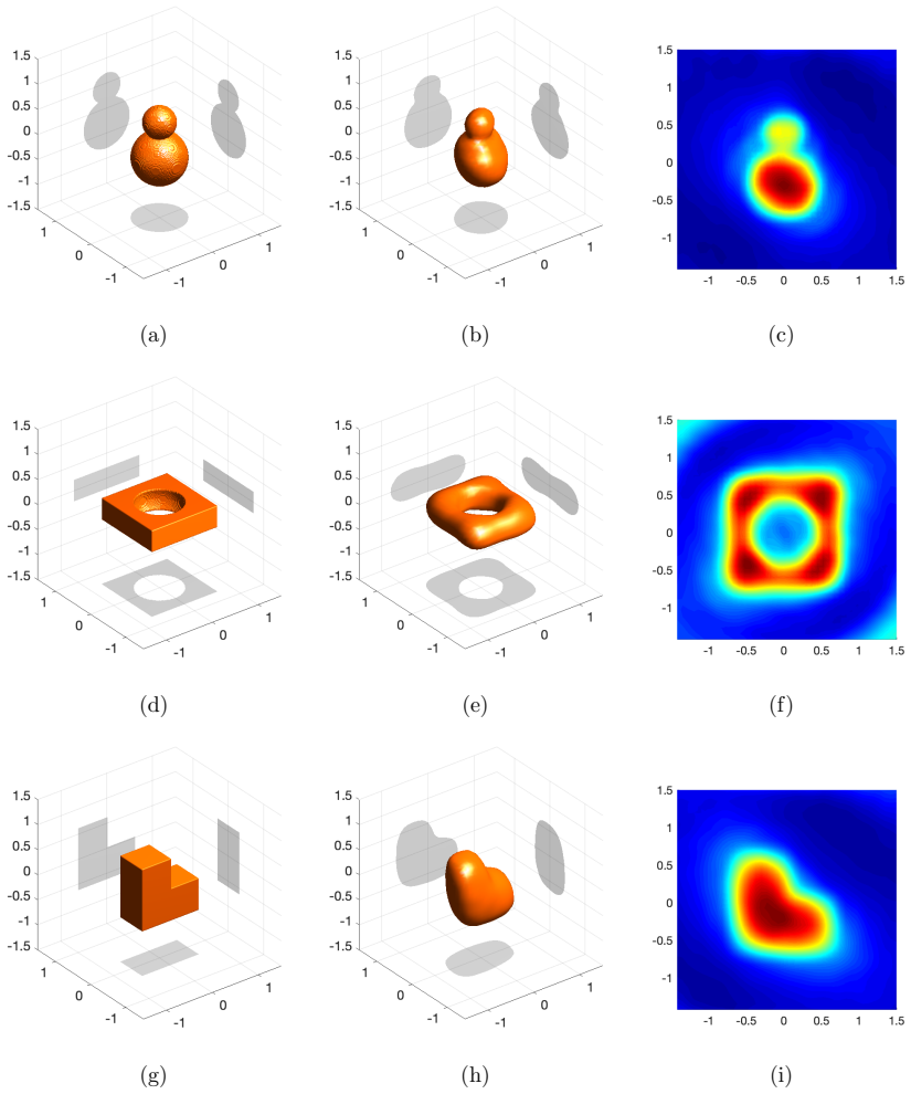
R. Potthast. A study on orthogonality sampling. Inverse Problems, 26:074015, 2010. 19 (a) (b) (c) (d) (e) (f) (g) (h) (i) Figure 4: Reconstruction of scatterers with more complicated shapes using OSM. There is 30% noise in the scattering data, Nˆx×Nd = 325× 325 andk = 12. The ...

2010

Pith tools

Reviewed August 14, 2026 · model on record in the stance chip above.

[1] [14]

A. Kirsch. The factorization method for Maxwell’s equations. Inverse Problems, 20:S117–S134, 2004

work page 2004

[2] [10]

H. Haddar. Analysis of some qualitative methods for inverse electromagnetic scat- tering problems. In Bermudez de Castro A., Valli A. (eds) Computational Elec- tromagnetism. Lecture Notes in Mathematics, vol 2148 , pages 191–240. Springer, Cham, 2014. 18

work page 2014

[3] [1]

Alzaalig

A.-M. Alzaalig. Direct Sampling Methods for Inverse Scattering Problems . PhD thesis, Michigan Technological University, 2017

work page 2017

[4] [2]

Bao and P

G. Bao and P. Li. Numerical solution of an inverse medium scattering problem for maxwell’s equations at ﬁxed frequency. J. Comput. Phys. , 228:4638–4648, 2009

work page 2009

[5] [3]

Cakoni, D

F. Cakoni, D. Colton, and P. Monk. The Linear Sampling Method in Inverse Electromagnetic Scattering. SIAM, 2011

work page 2011

[6] [4]

Cakoni, H

F. Cakoni, H. Haddar, and A. Lechleiter. On the factorization method for a far ﬁeld inverse scattering in the time domain. SIAM J. Math. Anal. , 51:854–872, 2019

work page 2019

[7] [5]

Cakoni and J

F. Cakoni and J. Rezac. Direct imaging of small scatterers using reduced time dependent data. J. Comput. Phys. , 338:371–387, 2017

work page 2017

[8] [6]

Q. Chen, H. Haddar, A. Lechleiter, and P. Monk. A sampling method for inverse scattering in the time domain. Inverse Problems, 26:085001, 2010

work page 2010