Purifying electron spectra from noisy pulses with machine learning using synthetic Hamilton matrices

Jan M. Rost; Sajal Kumar Giri; Ulf Saalmann

REVIEW 3 major objections 5 minor 34 references

Purifying electron spectra from noisy pulses with machine learning using synthetic Hamilton matrices

T0 review · 3 major / 5 minor · reviewed 2026-08-14 · deepseek-v4-flash

Challenge this review Re-run · record.json Download PDF Read on arXiv ↗ Review JSON

Pith's one-line read A deep neural network trained only on synthetic Hamilton matrices purifies noisy electron spectra from free-electron lasers, reproducing reference multi-peak structures for atoms and molecules never seen in training.

desk verdict Genuinely new dataset-generation idea (SHMs) and a fair generalization test to 3D systems, but the experimental transfer to SASE FELs remains unvalidated; worth serious review. read the letter →

arxiv 1908.02600 v2 pith:5WQB7DDL submitted 2019-08-07 physics.atom-ph

Sajal Kumar Giri , Ulf Saalmann , Jan M. Rost This is my paper · ORCID

classification physics.atom-ph

keywords photo-electronspectrafree-electronlasersSASEpulsessyntheticHamiltonmatricesdeepneuralnetworkpartial-coherencemethodmultiphotonionizationspectrumpurification

verification ladder T0 review T1 audit T2 compute T3 formal

The pith

A machine-rendered reading of the paper's core claim, the machinery that carries it, and where it could break.

The reading

The paper aims to show that electron spectra from fluctuating SASE free-electron laser pulses can be cleaned into the spectrum a Fourier-limited Gaussian pulse would produce, without ever training on the real system. The authors generate 200,000 training pairs by solving about ten million time-dependent Schrödinger equations for synthetic Hamilton matrices, randomized versions of a one-dimensional photoionization Hamiltonian, driven by random pulse realizations. They train a deep feedforward network to map averaged noisy spectra to the corresponding reference spectra. They demonstrate that the trained network reproduces multi-peak structures in three-dimensional helium and hydrogen-molecule-ion spectra that are completely absent from the averaged inputs, even though those systems were never part of the training data. This offers a route to extracting ideal-pulse spectra from inherently noisy FEL experiments.

What carries the argument

The central object is the synthetic Hamilton matrix $H_{kl}(t) = E_k + A_k f_l(t) V_k$, built by randomizing the diagonal energies $E_k$, the coupling elements $V_k$, and the field strengths $A_k$ around a one-dimensional photoionization Hamiltonian. With 20,000 such matrices and ten averaged noisy spectra per matrix, the paper generates 200,000 training pairs. Spectra are expanded in a basis of 60 harmonic-oscillator eigenfunctions, and the network maps the coefficients of noisy spectra to the coefficients of the corresponding reference spectrum. The random variation of the Hamilton matrices is what lets a network trained on cheap one-dimensional synthetic data generalize to full three-dimensional physical systems.

What would settle it

Measure the same target, for example helium at 21 eV, twice at a seeded free-electron laser: once with the fluctuating SASE-like mode and once with the coherent seed. Feed the averaged noisy spectrum to the network and compare its output with the measured seed spectrum; if they differ by more than the typical training error, the claim that SHM-trained purification transfers to experimental spectra is refuted.

Watch

Extended reading notes

Core claim

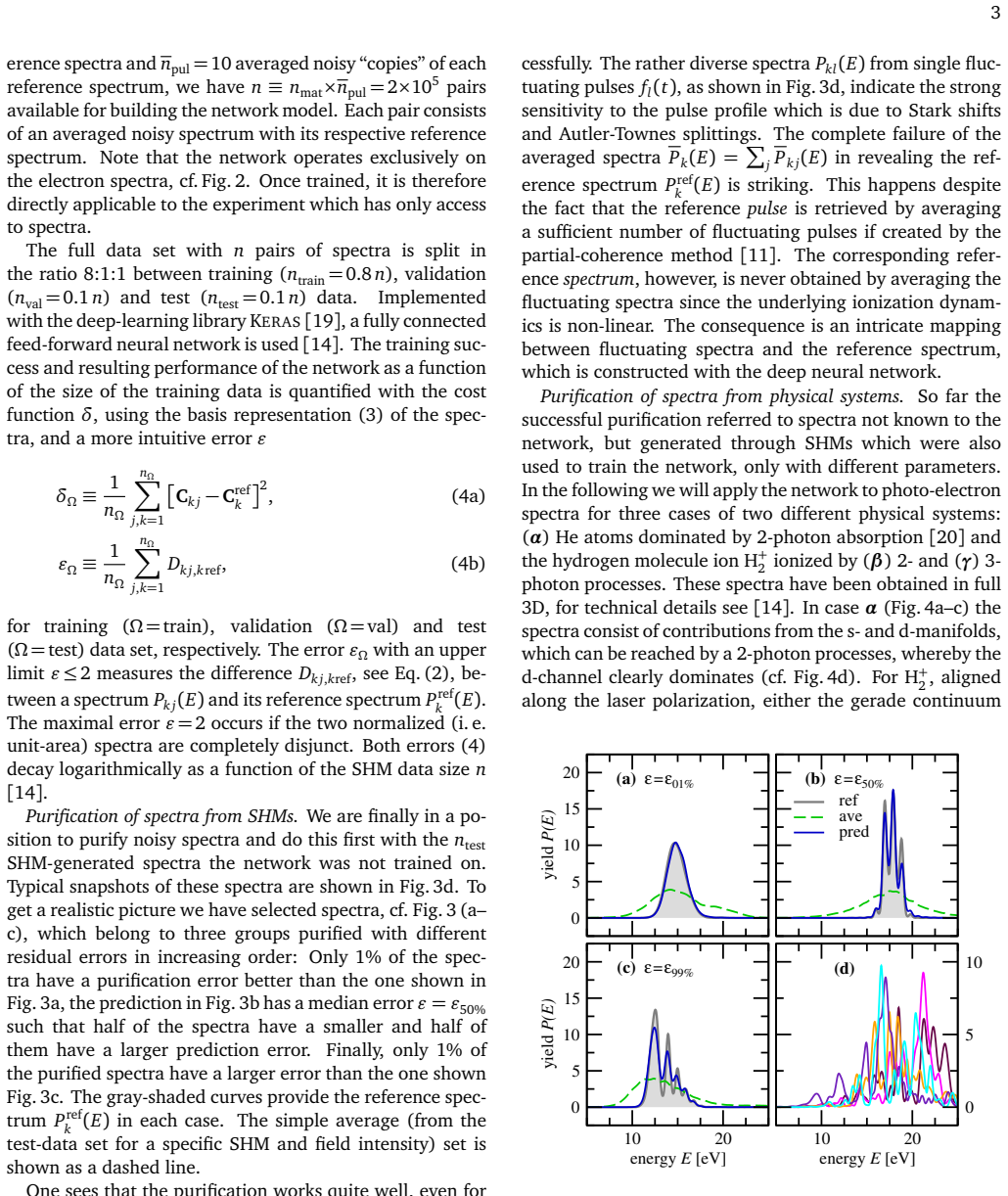
The central claim is that a deep network trained exclusively on spectra generated from synthetic Hamilton matrices is generic enough to purify realistic atomic and molecular photo-electron spectra dominated by resonant two- and three-photon ionization, where the purified spectrum is the one an ideal Fourier-limited Gaussian pulse would produce. The paper reports that for helium at 21 eV and for H2+ at 23 eV and 12 eV, at intensities from about $10^{14}$ to $10^{16}$ W/cm$^2$, the network maps averaged noisy spectra onto the reference spectra, recovering peak positions and fine structures that are invisible in the averages. Because the network operates only on the spectra and never on the Hamiltonian or the pulse, it can in principle be applied directly to experimental spectra.

Load-bearing premise

The load-bearing premise is that random variations of a one-dimensional ionization model cover the physics of real three-dimensional atoms and molecules, and that the model of pulse fluctuations matches the real ones at the free-electron laser; if either fails, the trained network will not purify experimental spectra.

Editorial extensions

If this is right

Experimental SASE FEL spectra could be purified without system-specific retraining, at least for few-photon ionization dominated by a single active electron.
Averaging many noisy spectra does not recover the reference spectrum because the ionization dynamics are nonlinear; the network performs a nonlinear inversion that simple averaging cannot.
The same synthetic-Hamilton-matrix strategy could be reused for other dynamical problems where deep networks need large training sets but exact simulations are expensive.
Purification can be conditioned on any chosen reference pulse, so the method could be adapted to different ideal pulse shapes or pulse parameters.

Reading between the lines

Editorial extensions of the paper, not claims the author makes directly.

An implication left implicit is that the same network might purify other observables, such as angular distributions or ion yields, as long as they are expressed in the same coefficient basis, since the network never sees the Hamiltonian.
A testable extension would be to condition the network on a non-Gaussian reference pulse, since the paper's pipeline allows the reference spectrum to be chosen arbitrarily.
The ability to randomize Hamiltonians suggests a broader recipe for data-scarce inverse problems: sample randomized surrogate Hamiltonians that preserve the qualitative level structure and nonlinearity, then train a network to invert the noise. The three physical test cases support this, but the boundary of the surrogate's validity is unknown.

Share X Bluesky LinkedIn Reddit HN

Signed reviews

No signed human review yet.

Editorial analysis

A structured set of objections, weighed in public.

Desk editor's note, referee report, and a circularity audit.

Desk Editor's Note

read the letter

The genuinely new thing here is the synthetic Hamilton matrix (SHM) construction. Instead of computing millions of expensive 3D TDSE spectra for training, the authors randomize energies, couplings, and field strengths around a fast 1D photoionization base. That lets them generate ~10^7 training spectra cheaply. This is a practical answer to the training-data bottleneck in ML-for-physics, and the SHM idea is likely to outlive this particular application. That's the main contribution.

What the paper does well: the testing protocol is honest. The network is trained on SHM spectra, tested on held-out SHM spectra, and then applied to full 3D TDSE spectra for He and H2+ at three intensities each — systems never shown during training. Fig. 4 shows the network recovering multi-peak reference structure that the averaged noisy spectra completely wash out. That is genuine evidence of transfer beyond the training family, not just interpolation. The errors reported on the SHM test set are also consistent with what the figures show.

The soft spot is the one the stress-test flags, and it's real. All training and test spectra use the same pulse statistics: T=3 fs, tau=0.5 fs, from the partial-coherence model. Real SASE pulses vary in coherence time, energy jitter, and noise correlations. Since the network inputs are only coefficients of the averaged spectrum, with no pulse parameters, any shift in pulse statistics is a distribution shift the network may not survive. The abstract's 'sufficiently generic' claim is stronger than the evidence: three 3D cases at one pulse-statistics point don't establish robustness to the full experimental range. To their credit, the authors explicitly propose a seeded-FEL benchmark as future work and acknowledge many-electron effects, so this is a stated limitation, not a hidden one. Minor point: no code or data is provided, which makes the SHM generation harder to reproduce, though the supplement covers the details.

Who is this for? Strong-field AMO and FEL experimentalists would use the method to get reference spectra from noisy SASE data; ML-for-physics people would study the SHM approach as a data-generation strategy. A serious referee should push for experimental validation or at least tests under varied pulse statistics, but the idea is sound enough to deserve referee time rather than a desk reject. Send it to peer review.

Referee Report

3 major / 5 minor

Summary. The manuscript proposes a deep neural network that maps an averaged, noisy photoelectron spectrum from a SASE FEL pulse train to the reference spectrum that would be produced by a Fourier-limited Gaussian pulse. Because ab initio training data are too expensive, the authors introduce synthetic Hamilton matrices (SHMs): random variations of energies and couplings around a one-dimensional photoionization model, propagated with the partial-coherence pulse model at fixed T = 3 fs and tau = 0.5 fs. They train a fully connected network on about 2e5 pairs of averaged noisy spectra and reference spectra, then test on held-out SHM spectra and on full 3D TDSE spectra for He and H2+ at several intensities and photon frequencies. The central claim is that the trained network is sufficiently generic to purify atomic and molecular spectra dominated by resonant two- or three-photon ionization without having been trained on those systems.

Significance. If the transferability claim holds, the SHM strategy is a valuable general recipe for generating large training sets in strong-field and attosecond physics, and the trained network could be a practical tool for FEL users who currently see only noisy averaged spectra. The paper's internal protocol is sound: the reference targets are computed independently by propagation with an ideal Gaussian pulse, the held-out SHM sets are not used in training, and the three 3D test systems are genuinely new to the network. The main contribution is conceptual rather than merely numerical, and the paper is clearly within the scope of physics.atom-ph.

major comments (3)

[Setting up networks with SHMs, item (ii), and Eq. (1)] The central transfer claim that the network is 'sufficiently generic' to purify experimental spectra is supported only by tests that use the same pulse-statistics model with fixed T = 3 fs and tau = 0.5 fs. All training data, held-out SHM spectra (Fig. 3), and the three 3D physical systems (Fig. 4) are generated with the same partial-coherence construction, and the network inputs contain no pulse parameters. A change in SASE coherence time, pulse-energy distribution, or noise correlations is therefore an unquantified distribution shift. The paper itself proposes a seeded-FEL benchmark only as future work, so the abstract's generalization claim is ahead of the evidence. I would ask for either a softened claim or additional tests with varied T, tau, and pulse-statistics models, ideally including a blinded experimental spectrum.
[Eq. (1) and item (ii), pulse-energy jitter] The treatment of pulse-energy jitter is incomplete. The text says the pulses 'additionally jitter in their pulse energy' but then normalizes every f_l(t) to unit pulse energy, and A_k in Eq. (1b) is fixed for all l of a given SHM. Thus the training data contain no pulse-energy jitter at all. Because the normalized spectrum in resonant few-photon ionization depends on the peak intensity through Rabi frequencies and Stark shifts, shot-to-shot energy jitter changes the normalized spectrum, not just its overall scale. If the network is intended for real SASE data, the authors should either include energy jitter in the training ensemble, for example by drawing random A_kl per realization, or explain explicitly why this fluctuation can be corrected or neglected experimentally.
[Introduction of SHMs, item (iii), and Fig. 4] The representativeness of the synthetic Hamilton matrices is asserted rather than demonstrated. The random variation in Eq. (1) around a 1D base is plausible, and the three successful 3D cases in Fig. 4 are encouraging, but they are only three systems, all using the same pulse model, and no quantitative measure is given of how well the SHM ensemble covers the subspace of realistic 3D few-photon ionization dynamics. A concrete test would be to train the network on SHM ensembles with different parameter ranges (number of states, coupling distribution, intensity range) and measure the resulting error on the same 3D benchmarks, or to project the 3D spectra into the network's feature space and compare with the SHM distribution. Without such a test, the 'sufficiently generic' statement in the abstract remains an extrapolation.

minor comments (5)

[Building and training the network, Eq. (4a)] The cost function as written compares the input noisy coefficients C_kj with the reference C_ref_k; the network output, presumably \tilde{C}_kj, is missing from the expression. As written, Eq. (4a) has no dependence on the trained mapping and cannot be the training error.
[Setting up networks with SHMs, items (iii) and (iv)] The symbol npul is used with two meanings: in item (iii) it is the number of noise realizations per SHM (500), while in item (iv) it is the number of averaged spectra (10). This makes Eq. (1) and the '10^3 fluctuating spectra' passage hard to follow; please use distinct symbols.
[Abstract and Fig. 2] The title and abstract say spectra are purified from noisy pulses, but the actual input to the network is an average over m = 200 pulses. The averaging requirement is central to the method and should be stated in the abstract.
[Normalization of spectra, item (iv)] All spectra are normalized to unit area before training and testing. This discards absolute-yield information; since the goal is a reference spectrum shape, this may be acceptable, but the authors should state explicitly what information is lost and why the network does not need it.
[Building and training the network] The main text refers to the supplement for the network architecture and all numerical details; for a standalone paper, please state at least the number of layers and neurons, the activation function, and the training epochs in the main text or in a table.

Circularity Check

0 steps flagged · score 2.0 of 10

No circularity: reference spectra are computed independently and physical systems are held out; self-citations are non-load-bearing.

full rationale

The derivation chain is not circular. Noisy inputs P_kj(E) are averaged from spectra generated with H_kl(t)=E_k + A_k f_l(t) V_k under fluctuating pulses, while the training target P_ref_k(E) is the spectrum of the same Hamilton matrix driven by the ideal reference pulse f_ref; the target is therefore an independent propagation result, not a fitted quantity. The cost function (4) and the 8:1:1 split provide held-out SHM test spectra, and the section on physical systems uses full-3D He and H2+ spectra computed with new random pulse realizations and never shown to the network, so the central transfer claim has an external benchmark within the paper. Self-citations (Refs [10], [14], [20]) supply physical context, technical details, or the He two-photon example, but none is invoked as a uniqueness theorem or as the source of training labels; the partial-coherence pulse model is cited to independent experimental work [11,12]. The main weakness, that one fixed pulse-statistics model (T=3 fs, tau=0.5 fs) may not cover other SASE statistics, is a generalization/correctness risk, and the manuscript itself defers experimental proof to future seeded-FEL benchmarks; this is not a reduction of the prediction to its inputs. Hence no circular step is exhibited.

Assumptions & free parameters 8 free parameters · 6 assumptions · 1 invented entities

The central claim relies on the SHM representativeness assumption and on the partial-coherence noise model; both are assumptions imported from the authors' construction or from prior work, not derived. Several numerical hyperparameters are chosen by hand. No new physical entity is postulated; SHMs are a computational construct with no external evidence.

free parameters (8)

nmat = 2×10^4
Number of synthetic Hamilton matrices selected by maximal mutual difference (Eq. 2); chosen to balance diversity and computational cost.
npul = 10
Number of averaged noisy spectra per reference used for training; chosen as compromise between ruggedness and effort (Sec. (iv)).
m = 200
Number of single-shot fluctuating spectra per average; larger m gives smoother averages but fewer training samples.
nbas_noisy = 60
Harmonic oscillator basis size for noisy spectra in Eq. (3); chosen sufficiently large to represent averaged spectra.
nbas_reference = 40
Basis size for reference spectra; chosen as sufficient for smooth spectra.
pulse_T_tau = T=3 fs, tau=0.5 fs
Characteristic duration and coherence time of fluctuating pulses in the partial-coherence model.
intensity_range = 5×10^15 to 5×10^16 W/cm^2
Range of field strengths for synthetic Hamilton matrices, corresponding to non-perturbative few-photon ionization.
network_hyperparameters = not specified in main text
Architecture, layer sizes, regularization, and training details deferred to the supplemental material.

assumptions (6)

domain assumption The partial-coherence method (Refs [11,12]) accurately models SASE FEL pulse fluctuations.
Used to generate all noisy pulse realizations; if the model mismatches real SASE statistics, the trained network sees the wrong noise distribution.
ad hoc to paper Randomly varied synthetic Hamilton matrices around a 1D base are representative of real few-photon ionization systems.
Central enabling assumption for generalization; not derived, supported only by three 3D test cases.
domain assumption Single-active-electron TDSE describes the target photoionization processes.
All training and test spectra come from single-active-electron TDSE; many-electron effects are acknowledged as a limitation.
domain assumption Pulses and spectra can be normalized to unit energy in experiment with gas monitor detectors.
Training assumes unit pulse energy and unit-area spectra; experiment must match this.
domain assumption Harmonic oscillator basis with nbas=60 (noisy) and 40 (reference) represents spectra accurately.
Truncation error in Eq. (3) is not quantified in the main text.
ad hoc to paper A network trained on SHM spectra will generalize to real atomic and molecular spectra.
Contrasted with the standard i.i.d. assumption; only three test cases support it.

invented entities (1)

synthetic Hamilton matrices (SHMs)
purpose: Random matrices of field-free energies, couplings, and field strengths replacing a full physical Hamiltonian for training-data generation.
No external validation outside this paper; the 3D test cases are internal evidence only.

how reviews work

0 comments

Cite this review

Pith. "Pith review of Purifying electron spectra from noisy pulses with machine learning using synthetic Hamilton matrices." pith.science (2026). https://pith.science/paper/5WQB7DDL

@misc{pith2026190802600,
  author       = {Pith},
  title        = {Pith review of: Purifying electron spectra from noisy pulses with machine learning using synthetic Hamilton matrices},
  year         = {2026},
  howpublished = {\url{https://pith.science/paper/5WQB7DDL}},
  note         = {Machine review of arXiv:1908.02600}
}

read the original abstract

Photo-electron spectra obtained with intense pulses generated by free-electron lasers through self-amplified spontaneous emission are intrinsically noisy and vary from shot to shot. We extract the purified spectrum, corresponding to a Fourier-limited pulse, with the help of a deep neural network. It is trained on a huge number of spectra, which was made possible by an extremely efficient propagation of the Schr\"odinger equation with synthetic Hamilton matrices and random realizations of fluctuating pulses. We show that the trained network is sufficiently generic such that it can purify atomic or molecular spectra, dominated by resonant two- or three-photon ionization, non-linear processes which are particularly sensitive to pulse fluctuations. This is possible without training on those systems.

Figures

Figures reproduced from arXiv: 1908.02600 by the authors.

**Figure 2.** FIG. 2. Building a network with synthetic Hamilton matrices and [PITH_FULL_IMAGE:figures/full_fig_p002_2.png] view at source ↗

**Figure 3.** FIG. 3. Photo-electron spectra from the SHM test-data set. The [PITH_FULL_IMAGE:figures/full_fig_p003_3.png] view at source ↗

Figures from the paper (1 more)

**Figure 4.** Figure 4: FIG. 4. Photo-electron spectra for the He atom (a–d) and the H [PITH_FULL_IMAGE:figures/full_fig_p004_4.png]

Discussion (0). Continue with ORCID to comment.

Reference graph

Works this paper leans on

34 extracted references · 32 canonical work pages

[1]

Dunjko and H

V . Dunjko and H. J. Briegel,Machine learning & artiﬁcial in- telligence in the quantum domain: A review of recent progress. Rep. Prog. Phys. 81, 074001 (2018)

work page 2018
[2]

Mehta, M

P . Mehta, M. Bukov, C.-H. Wang, A. G. R. Day , C. Richardson, C. K. Fisher, and D. J. Schwab, A high-bias, low-variance in- troduction to machine learning for physicists. Phys. Rep. 810, 1 (2019)

work page 2019
[3]

Carleo, I

G. Carleo, I. Cirac, K. Cranmer, L. Daudet, M. Schuld, N. Tishby , L. Vogt-Maranto, and L. Zdeborová,Machine learning and the physical sciences . arXiv:1903.10563 (2019), arXiv: 1903.10563

arXiv 2019
[4]

Carleo and M

G. Carleo and M. Troyer, Solving the quantum many-body problem with artiﬁcial neural networks . Science 355, 602 (2017)

work page 2017
[5]

Sanchez-Gonzalez et al., Accurate prediction of X-ray pulse properties from a free-electron laser using machine learning

A. Sanchez-Gonzalez et al., Accurate prediction of X-ray pulse properties from a free-electron laser using machine learning . Nat. Commun. 8, ncomms15461 (2017)

work page 2017
[6]

Rogus and M

D. Rogus and M. Lewenstein, Resonant ionisation by smooth laser pulses. J. Phys. B 19, 3051 (1986)

work page 1986
[7]

S. H. Autler and C. H. Townes,Stark effect in rapidly varying ﬁelds. Phys. Rev. 100, 703 (1955)

work page 1955
[8]

Meier and V

C. Meier and V . Engel,Interference structure in the photoelec- tron spectra obtained from multiphoton ionization of Na2 with a strong femtosecond laser pulse . Phys. Rev. Lett. 73, 3207 (1994)

work page 1994

Show all 34 references

[9]

P . V . Demekhin and L. S. Cederbaum,Coherent intense reso- nant laser pulses lead to interference in the time domain seen in the spectrum of the emitted particles. Phys. Rev. A86, 063412 (2012)

2012
[10]

Baghery , U

M. Baghery , U. Saalmann, and J. M. Rost, Essential condi- tions for dynamic interference . Phys. Rev. Lett. 118, 143202 (2017)

2017
[11]

Pfeifer, Y

T . Pfeifer, Y. Jiang, S. Düsterer, R. Moshammer, and J. Ullrich, Partial-coherence method to model experimental free-electron laser pulse statistics. Opt. Lett. 35, 3441 (2010)

2010
[12]

Moshammer et al., Second-order autocorrelation of XUV FEL pulses via time-resolved two-photon single ionization of He

R. Moshammer et al., Second-order autocorrelation of XUV FEL pulses via time-resolved two-photon single ionization of He. Opt. Express 16, 21698 (2011)

2011
[13]

Tiedtke et al., Gas detectors for X-ray lasers

K. Tiedtke et al., Gas detectors for X-ray lasers. J. Appl. Phys. 103, 094511 (2008)

2008
[14]

See Supplemental Material [url] for details on generating laser pulses, propagating the time-dependent Schrödinger equation and training of artiﬁcial neural networks, which in- cludes additional references [27–34]
[15]

Tao and A

L. Tao and A. Scrinzi,Photo-electron momentum spectra from minimal volumes: the time-dependent surface ﬂux method . New J. Phys. 14, 013021 (2012); A. Scrinzi, t-SURFF: Fully differential two-electron photo-emission spectra. New J. Phys. 14, 085008 (2012)

2012
[16]

Mosert and D

V . Mosert and D. Bauer,Photoelectron spectra with Qprop and t-SURFF. Comput. Phys. Commun. 207, 452 (2016)

2016
[17]

Patchkovskii and H

S. Patchkovskii and H. G. Muller, Simple, accurate, and ef- ﬁcient implementation of 1-electron atomic time-dependent Schrödinger equation in spherical coordinates. Comput. Phys. Commun. 199, 153 (2016)

2016
[18]

reference spectrum

We will use the terms “reference spectrum” and “ﬂuctuating spectrum” to refer to a “spectrum from a reference pulse” and a “spectrum from a ﬂuctuating pulse”, respectively . We never deal with the spectral representation of the pulse itself
[19]

Chollet,Keras: The Python deep learning library

F . Chollet,Keras: The Python deep learning library. https://keras.io (2015)

2015
[20]

Saalmann, S

U. Saalmann, S. K. Giri, and J. M. Rost, Adiabatic passage to the continuum: Controlling ionization with chirped laser pulses. Phys. Rev. Lett. 121, 153203 (2018)

2018
[21]

Amann et al., Demonstration of self-seeding in a hard-X-ray free-electron laser

J. Amann et al., Demonstration of self-seeding in a hard-X-ray free-electron laser. Nat. Photon. 6, 693 (2012)

2012
[22]

Allaria et al., Highly coherent and stable pulses from the FERMI seeded free-electron laser in the extreme ultraviolet

E. Allaria et al., Highly coherent and stable pulses from the FERMI seeded free-electron laser in the extreme ultraviolet. Nat. Photon. 6, 699 (2012)

2012
[23]

Allaria et al.,Two-stage seeded soft-X-ray free-electron laser

E. Allaria et al.,Two-stage seeded soft-X-ray free-electron laser. Nat. Photon. 7, 913 (2013)

2013
[24]

P . R. Ribiˇc et al., Coherent soft X-ray pulses from an echo- enabled harmonic generation free-electron laser. Nat. Photon. 13, 555 (2019)

2019
[25]

Rohringer and R

N. Rohringer and R. Santra, X-ray nonlinear optical processes using a self-ampliﬁed spontaneous emission free-electron laser. Phys. Rev. A 76, 033416 (2007)

2007
[26]

G. M. Nikolopoulos and P . Lambropoulos, Effects of free- electron-laser ﬁeld ﬂuctuations on the frequency response of driven atomic resonances. Phys. Rev. A 86, 033420 (2012)

2012
[27]

Geloni, E

G. Geloni, E. Saldin, L. Samoylova, E. Schneidmiller, H. Sinn, Th Tschentscher, and M. Yurkov, Coherence properties of the European XFEL. New J. Phys. 12, 035021 (2010)

2010
[28]

X. M. Tong and C. D. Lin, Empirical formula for static ﬁeld ionization rates of atoms and molecules by lasers in the barrier- suppression regime. J. Phys. B 38, 2593 (2005)

2005
[29]

L. D. Landau and E. M. Lifschitz, Quantum mechanics. Perg- amon Press, Oxford 1989

1989
[30]

Glorot, A

X. Glorot, A. Bordes, and Y. Bengio,Deep sparse rectiﬁer neu- ral networks. PMLR 15, 315 (2011)

2011
[31]

Glorot and Y

X. Glorot and Y. Bengio,Understanding the difﬁculty of train- ing deep feedforward neural networks. PMLR 9, 249 (2010)

2010
[32]

D. P . Kingma and J. L. Ba, ADAM: A method for stochastic optimization. arXiv:1412.6980 [cs] (2017)

2017 arXiv
[33]

M. Li, T . Zhang, Y. Chen, and A. J. Smola,Efﬁcient mini-batch training for stochastic optimization in Proceedings of the 20th ACM SIGKDD Conference, 661 (2014)

2014
[34]

Srivastava, G

N. Srivastava, G. Hinton, A. Krizhevsky , I. Sutskever, and R. Salakhutdinov, Dropout: A simple way to prevent neural networks from overﬁtting. JMLR 15, 1929 (2014)

2014

Pith tools

Reviewed August 14, 2026 · model on record in the stance chip above.

[1] [1]

Dunjko and H

V . Dunjko and H. J. Briegel,Machine learning & artiﬁcial in- telligence in the quantum domain: A review of recent progress. Rep. Prog. Phys. 81, 074001 (2018)

work page 2018

[2] [2]

Mehta, M

P . Mehta, M. Bukov, C.-H. Wang, A. G. R. Day , C. Richardson, C. K. Fisher, and D. J. Schwab, A high-bias, low-variance in- troduction to machine learning for physicists. Phys. Rep. 810, 1 (2019)

work page 2019

[3] [3]

Carleo, I

G. Carleo, I. Cirac, K. Cranmer, L. Daudet, M. Schuld, N. Tishby , L. Vogt-Maranto, and L. Zdeborová,Machine learning and the physical sciences . arXiv:1903.10563 (2019), arXiv: 1903.10563

arXiv 2019

[4] [4]

Carleo and M

G. Carleo and M. Troyer, Solving the quantum many-body problem with artiﬁcial neural networks . Science 355, 602 (2017)

work page 2017

[5] [5]

Sanchez-Gonzalez et al., Accurate prediction of X-ray pulse properties from a free-electron laser using machine learning

A. Sanchez-Gonzalez et al., Accurate prediction of X-ray pulse properties from a free-electron laser using machine learning . Nat. Commun. 8, ncomms15461 (2017)

work page 2017

[6] [6]

Rogus and M

D. Rogus and M. Lewenstein, Resonant ionisation by smooth laser pulses. J. Phys. B 19, 3051 (1986)

work page 1986

[7] [7]

S. H. Autler and C. H. Townes,Stark effect in rapidly varying ﬁelds. Phys. Rev. 100, 703 (1955)

work page 1955

[8] [8]

Meier and V

C. Meier and V . Engel,Interference structure in the photoelec- tron spectra obtained from multiphoton ionization of Na2 with a strong femtosecond laser pulse . Phys. Rev. Lett. 73, 3207 (1994)

work page 1994