REVIEW 3 major objections 7 minor 48 references
Stability Analysis of Reservoir Computers Dynamics via Lyapunov Functions
T0 review · 3 major / 7 minor · reviewed 2026-08-14 · deepseek-v4-flash
Pith's one-line read A Lyapunov comparison identifies a ball of guaranteed stability around a reservoir computer's fixed point, and training error is lowest inside that ball.
desk verdict Solid continuous-time stability criterion for reservoir computers, but the discrete-time proof has a load-bearing norm/spectral-radius gap that needs fixing before the c-region claims for nonnormal adjacency matrices can stand. read the letter →
The pith
A machine-rendered reading of the paper's core claim, the machinery that carries it, and where it could break.
The reading
What carries the argument
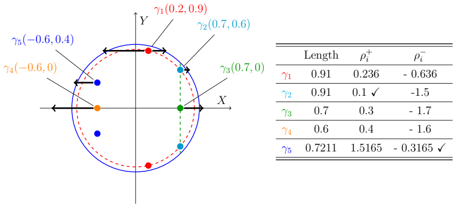
The named object is the $c(\theta)$-region: the ball of radius $c$ around the fixed point inside which the Lyapunov function certifies stability. What carries the argument is the scalar bound $K^*(c,\theta)$, obtained by solving $\min K$ subject to $r_i f(r_i;\theta) - K r_i^2 \le 0$ on $[-c,c]$; the optimum is the largest of $f(c)/c$, $f(-c)/(-c)$, $f'(0)$, and $f(r^*)/r^*$ at interior stationary points of the ratio. Stability in continuous time reduces to $K^*(c,\theta) \le -\alpha_{\max}(A_s)$, decoupling node dynamics from network topology. In discrete time, the same ratio is squeezed from both sides, $K_-^* \le f(r_i;\theta)/r_i \le K_+^*$, and the admissible corridor is set by the two eigenvalues of $A$ whose real parts are closest to the unit circle; the stability radius is $c_{\max} = \min\{c^+_{\max}, c^-_{\max}\}$.
What would settle it
Construct a 2-node discrete reservoir with $f(r)=0$ and adjacency matrix $A = [[0.9, 1], [0, 0.9]]$. All eigenvalues equal 0.9, so with $K=0$ the paper's condition holds, but the matrix norm exceeds 1; starting inside the unit ball on the top singular-vector direction, the state norm immediately grows past 1, so the predicted invariant ball is not invariant. That observation settles whether the discrete-time $c$-region theorem holds as stated.
Extended reading notes
Core claim
The paper's central claim is that, for a given unforced reservoir computer with a fixed point shifted to the origin, a scalar comparison function can certify nonlinear stability on an explicit ball. In continuous time, let $K^*(c,\theta)$ be the smallest $K$ such that $r_i f(r_i;\theta) \le K r_i^2$ for all $r_i \in [-c,c]$; then every trajectory starting in the ball $\|r\| \le c$ converges to the origin when $K^*(c,\theta) \le -\alpha_{\max}(A_s)$, where $A_s$ is the symmetric part of the adjacency matrix. In discrete time the same idea uses $V(r)=\|r\|$ and a corridor of two bounds $K_-^* \le f(r_i;\theta)/r_i \le K_+^*$, admissible when they fall between the shifts toward the unit circle set by the nearest eigenvalues. The paper then reports that in simulations the training error of a 100-node reservoir is markedly lower exactly in the parameter region where these global-stability conditions hold, and that for polynomial node dynamics the reservoir works when the polynomial contains both an odd and an even power, with the quadratic coefficient playing a distinctive role.
Load-bearing premise
The discrete-time argument assumes that squeezing every ratio $f(r_i)/r_i$ between the same two constants is enough to bound the norm of the whole map, and that checking eigenvalues alone controls that norm; this requires the adjacency matrix's eigenvectors to be mutually perpendicular, a condition the paper never states.
Editorial extensions
If this is right
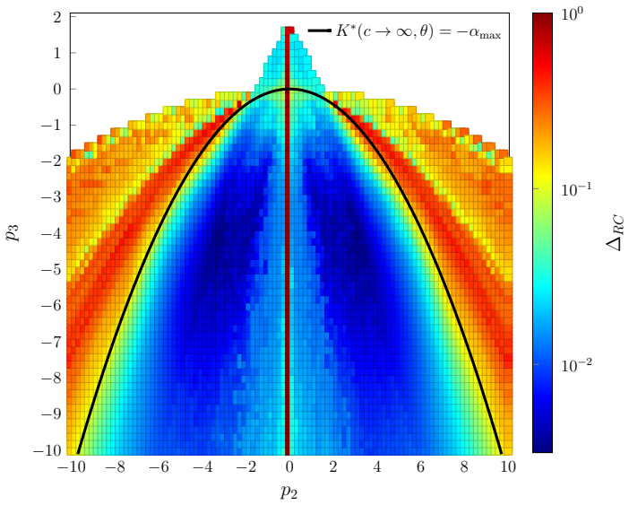
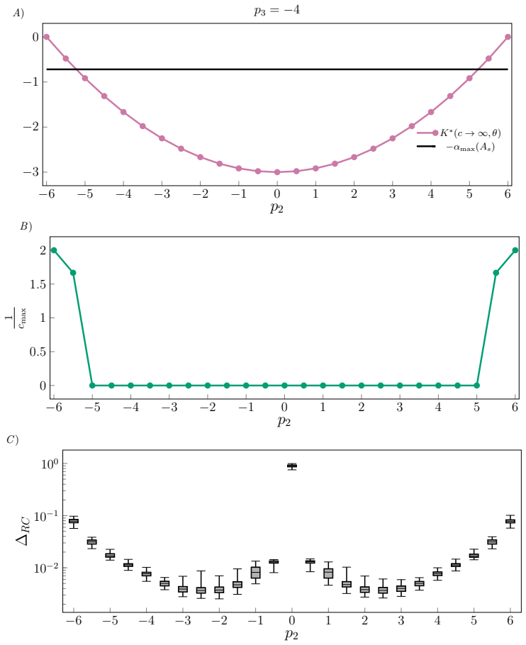
- In continuous-time polynomial reservoirs, the curve $K^*(\infty,\theta)=-\alpha_{\max}(A_s)$ marks the boundary below which training error is low; parameters above it risk divergence or convergence to a different attractor.
- The $c(\theta)$-region rule separates nodal dynamics from network topology, so a designer can enlarge the stable region by adjusting $K^*$, the node nonlinearity, or by adjusting $\alpha_{\max}$, the coupling structure.
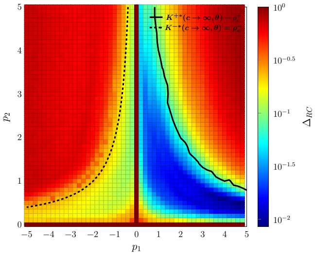
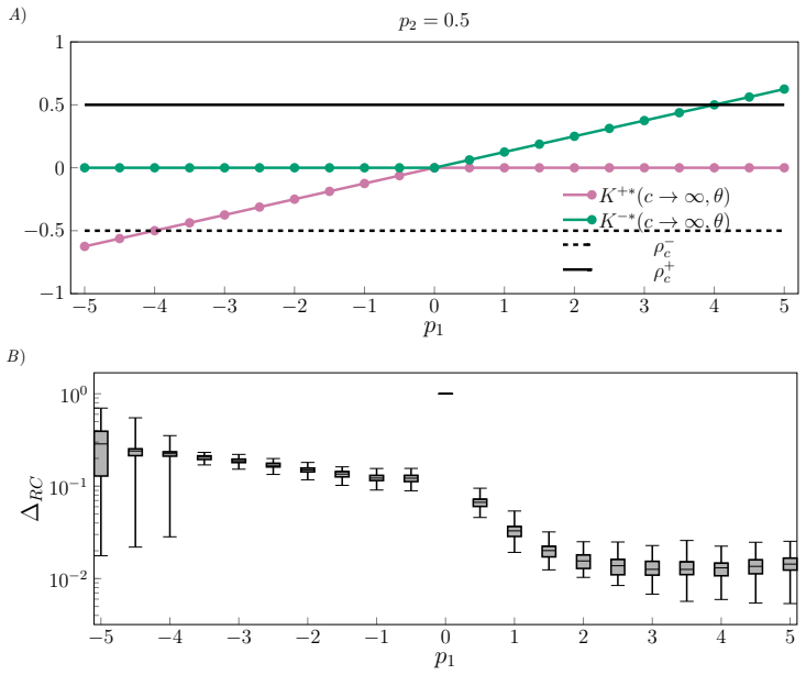
- For discrete-time sigmoid reservoirs, global stability holds between the curves $K_+^*=\rho_c^+$ and $K_-^*=\rho_c^-$, and the training error is small only inside that corridor.
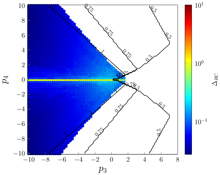
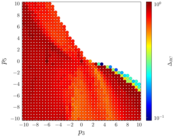
- Polynomial node functions with only odd powers, such as linear, cubic, and fifth-order terms, perform poorly; a nonzero even-power coefficient is required, with a zero quadratic coefficient producing training error near one.
- Because the analysis is input independent, a reservoir stabilized at the origin will remain near the operating point for any bounded input signal, not just for the training signal.
Reading between the lines
- Extension: the same $K^*/\alpha_{\max}$ split suggests a direct design optimization: maximize the radius $c_{\max}$ by tuning node parameters and adjacency weights separately, since the two contributions decouple.
- Extension: the discrete-time criterion should be tightened to use a genuine norm bound, for example the induced 2-norm, rather than eigenvalues alone for non-normal adjacency matrices; this would shrink the predicted $c_{\max}$ and can be checked against direct simulation.
- Extension: the odd/even-power requirement may generalize to a necessary condition for polynomial activations in reservoirs: an even power breaks sign symmetry, and this could be tested on higher-degree polynomials and different reservoir topologies.
- Extension: the basin radius could be converted into an input-amplitude bound for the forced system: normalize inputs so the driven trajectory stays inside $D(c_{\max})$, giving a tighter but input-specific performance guarantee.
Signed reviews
Editorial analysis
A structured set of objections, weighed in public.
Referee Report
Summary. The paper proposes a Lyapunov-based method to certify nonlinear stability of reservoir computers around a fixed point, for both continuous-time and discrete-time dynamics. For continuous time, the authors derive a sufficient condition K*(c,theta) <= -alpha_max(A_s), where K* is the maximum of f(r)/r on [-c,c] and alpha_max is the largest eigenvalue of the symmetric part of the adjacency matrix. For discrete time, they propose a condition involving eigenvalues of the adjacency matrix and bounds K- and K+ on f(r)/r, and they use these conditions to draw parameter-space stability boundaries. Numerically, the paper reports training errors for continuous-time polynomial reservoirs and discrete-time sigmoid reservoirs, finding that training error tends to be lower in the analytically predicted globally stable parameter region.
Significance. If the discrete-time arguments were correct, the paper would offer a simple, input-independent design rule for choosing reservoir parameters that guarantee stability, along with an interesting empirical link between the predicted global stability region and low training error. The continuous-time sufficient condition is derived cleanly, and the decoupling between nodal dynamics and network topology is a useful and clearly presented idea. The paper's numerical validation with Lorenz and Duffing signals is a genuine strength, and the analytical boundary curves in the figures are not fits to the error data. However, the discrete-time stability result currently rests on an invalid norm inequality and on an unjustified replacement of an operator norm by a spectral radius, so the discrete-time portion of the central claim is not supported as written.
major comments (3)
- [Section II.B.1, Eq. (19)] The inequality ||f(r)+Ar|| <= ||K(c,theta) r + Ar|| is asserted to follow from the componentwise bound f_i(r_i) <= K(c,theta) r_i, but this implication is false. For example, take K=1, r=(1,-1), and f(r)=(1,-100); each component satisfies f_i <= K r_i (1<=1 and -100<=-1), yet ||f(r)|| = sqrt(10001) > ||K r|| = sqrt(2). Since this norm inequality is the step that reduces the Lyapunov decrement to a check on the linear operator K I + A, the discrete-time stability condition is not established by the given argument.
- [Section II.B.1, Eqs. (20a)-(20b)] The passage from |K + gamma_i| <= 1 for every eigenvalue gamma_i of A to the operator norm bound ||K I + A||_2 <= 1 is valid only for normal matrices, and the random adjacency matrices constructed in Section III are generally non-normal. A concrete counterexample is A = [[0,2],[0,0]] with K=0: the spectral radius is 0, yet ||A||_2 = 2, so the Lyapunov function V(r)=||r|| can increase even though the eigenvalue condition holds. Consequently, the discrete-time c-region and the boundary curves K+*(c,theta)=rho_c^+ and K-*(c,theta)=rho_c^- in Figs. 8-9 are not justified by the arguments provided.
- [Section II.B.2, Eqs. (37)-(41)] In the non-homogeneous case, the reduction to scalar bounds K-* = min_i K_i^-* and K+* = max_i K_i^+* is not sufficient for the norm inequality needed with V(r)=||r||. The actual map involves a state-dependent diagonal matrix D(r) = diag(f_i(r_i)/r_i), and bounding each entry of D(r) by the global scalars K-* and K+* does not control ||D(r)+A||_2 when A is non-normal. Since the sigmoid example in Section III.C has node-dependent fixed points q_i* and hence node-dependent K_i^+* and K_i^-*, the discrete-time numerical boundaries in Fig. 8 also rely on this unjustified scalarization.
minor comments (7)
- [Section II.A.2] The text states that the origin is linearly stable if the largest real part of the eigenvalues of (A - p1 I) is negative; the linearization of Eq. (13) at the origin is A + p1 I, so this appears to be a sign error that should be corrected.
- [Eq. (20a)] The notation |K I + A| is undefined; if it denotes a determinant, it is not the induced norm needed for the Lyapunov argument, and if it denotes the matrix of absolute values, it is not what is used in Eq. (20b).
- [Eq. (14)] The formula for the interior critical point r* = -p2/(2p3) is singular when p3 = 0, a case that occurs in the parameter scans of Figs. 3-4; the handling of the case p3 = 0 should be stated explicitly.
- [Introduction] The claim that global asymptotic stability of the unforced system implies stable behavior under any bounded input is not true for general nonlinear systems; the authors should either prove an input-to-state stability property or soften this statement to avoid overclaiming.
- [Section III.A, Eqs. (51)-(52)] The training error formula Delta_RC = <Omega k - g> / <g> is confusing because <X> is later defined as the RMS value; please define the normalized RMS error explicitly.
- [Fig. 2 caption] The caption contains an apparent typo ('closest to the positive side of the unit circle Wis'), and the definitions of rho_i^+ and rho_i^- in the caption are hard to follow without repeating Eq. (22).
- [Section III.C, Eqs. (44)-(45)] The indices in the sums involving A_{ij} q*_i and A_{ij} q*_j appear inconsistent; the fixed-point shift should be checked to ensure the transformed dynamics is written correctly.
Circularity Check
No significant circularity: the stability region is derived analytically from the reservoir dynamics, and the training error is an independent benchmark.
full rationale
The paper's central stability condition is derived from the reservoir dynamics and a quadratic-norm Lyapunov function: Eq. (6b) follows from bounding r_i f(r_i) by K(c, θ) r_i^2 and using the largest eigenvalue of the symmetric part of A, while the optimal K*(c, θ) is obtained from the optimization in Eqs. (7)-(10) rather than from training-error data. The reported boundary curves (Figs. 3, 4, and 8) are evaluations of K*(c→∞, θ) = −α_max(A_s) or K±*(c→∞, θ) = ρ±, which are analytical expressions in the nodal parameters and the eigenvalues of A. The training error Δ_RC is computed by an independent least-squares fit (Eqs. (48)-(52)) and then compared with the analytically predicted stable region; the paper never fits K* or c_max to the error map. There are no load-bearing self-citations: the cited items are standard Lyapunov theory and external reservoir-computing papers, and no uniqueness theorem or prior-work ansatz is invoked to force the chosen form. The discrete-time derivation's replacement of a matrix norm by its spectral radius in Eq. (20) is a mathematical gap for non-normal A, but it is not circular—it does not assume the conclusion and does not make the prediction equivalent to its inputs. Hence no circular step meets the quoted-evidence standard.
Assumptions & free parameters
free parameters (6)
- p1 (linear coefficient) =
-3 in continuous-time simulations
- p2 (quadratic coefficient) =
scanned, e.g., -10 to 10 in Figs. 3-4; p2=0 is the failure case
- p3 (cubic coefficient) =
scanned, e.g., -10 to 10 in Fig. 3; p3=-4 in Fig. 7
- p4 (quartic coefficient) =
scanned in Fig. 5; zero elsewhere
- p5 (quintic coefficient) =
scanned in Fig. 6; zero elsewhere
- adjacency spectral normalization =
0.5
assumptions (6)
- standard math Lyapunov stability theorems: existence of V with V>0 and V-dot<0 on D(c) implies asymptotic stability
- domain assumption The origin is a fixed point and is linearly stable for the unforced dynamics
- domain assumption The reservoir nodes are homogeneous (same function f and same parameter theta) for the main derivations
- domain assumption For non-homogeneous dynamics, any nonzero fixed point can be moved to the origin by coordinate transformation
- ad hoc to paper Global asymptotic stability of the unforced system implies stable behavior under any bounded input
- ad hoc to paper The discrete-time norm bound ||f(r)+Ar|| <= ||K r+Ar|| follows from f_i(r_i) <= K r_i, and ||K I + A|| is controlled by the eigenvalues of A
Cite this review
Pith. "Pith review of Stability Analysis of Reservoir Computers Dynamics via Lyapunov Functions." pith.science (2026). https://pith.science/paper/6AFXRIIC
@misc{pith2026190804411,
  author       = {Pith},
  title        = {Pith review of: Stability Analysis of Reservoir Computers Dynamics via Lyapunov Functions},
  year         = {2026},
  howpublished = {\url{https://pith.science/paper/6AFXRIIC}},
  note         = {Machine review of arXiv:1908.04411}
}
read the original abstract
A Lyapunov design method is used to analyze the nonlinear stability of a generic reservoir computer for both the cases of continuous-time and discrete-time dynamics. Using this method, for a given nonlinear reservoir computer, a radial region of stability around a fixed point is analytically determined. We see that the training error of the reservoir computer is lower in the region where the analysis predicts global stability but is also affected by the particular choice of the individual dynamics for the reservoir systems. For the case that the dynamics is polynomial, it appears to be important for the polynomial to have nonzero coefficients corresponding to at least one odd power (e.g., linear term) and one even power (e.g., quadratic term).
Figures

Figures from the paper (6 more)

Reference graph
Works this paper leans on
-
[1]
Herbert Jaeger. The “echo state” approach to analysing and training recurrent neural networks-with an erratum note. Bonn, Germany: German National Research Center for Information Technology GMD Technical Report , 148(34):13, 2001
work page 2001
-
[2]
An overview of reservoir computing: theory, applications and implementations
Benjamin Schrauwen, David Verstraeten, and Jan Van Campenhout. An overview of reservoir computing: theory, applications and implementations. In Proceedings of the 15th european symposium on artificial neural networks. p. 471-482 2007 , pages 471--482, 2007
work page 2007
-
[3]
a ger, Wolfgang Maass, and Henry Markram. The
Thomas Natschl \"a ger, Wolfgang Maass, and Henry Markram. The" liquid computer": A novel strategy for real-time computing on time series. Special issue on Foundations of Information Processing of TELEMATIK , 8(ARTICLE):39--43, 2002
work page 2002
-
[4]
Real-time computing without stable states: A new framework for neural computation based on perturbations
Wolfgang Maass, Thomas Natschl \"a ger, and Henry Markram. Real-time computing without stable states: A new framework for neural computation based on perturbations. Neural computation , 14(11):2531--2560, 2002
2002
-
[5]
Photonic nonlinear transient computing with multiple-delay wavelength dynamics
Romain Martinenghi, Sergei Rybalko, Maxime Jacquot, Yanne K Chembo, and Laurent Larger. Photonic nonlinear transient computing with multiple-delay wavelength dynamics. Physical review letters , 108(24):244101, 2012
work page 2012
-
[6]
Parallel photonic information processing at gigabyte per second data rates using transient states
Daniel Brunner, Miguel C Soriano, Claudio R Mirasso, and Ingo Fischer. Parallel photonic information processing at gigabyte per second data rates using transient states. Nature communications , 4:1364, 2013
work page 2013
-
[7]
Information processing via physical soft body
Kohei Nakajima, Helmut Hauser, Tao Li, and Rolf Pfeifer. Information processing via physical soft body. Scientific reports , 5:10487, 2015
work page 2015
-
[8]
Photonic delay systems as machine learning implementations
Michiel Hermans, Miguel C Soriano, Joni Dambre, Peter Bienstman, and Ingo Fischer. Photonic delay systems as machine learning implementations. Journal of Machine Learning Research , 2015
work page 2015
Show all 48 references
-
[9]
High-performance photonic reservoir computer based on a coherently driven passive cavity
Quentin Vinckier, Fran c ois Duport, Anteo Smerieri, Kristof Vandoorne, Peter Bienstman, Marc Haelterman, and Serge Massar. High-performance photonic reservoir computer based on a coherently driven passive cavity. Optica , 2(5):438--446, 2015
2015
-
[10]
Fully analogue photonic reservoir computer
Fran c ois Duport, Anteo Smerieri, Akram Akrout, Marc Haelterman, and Serge Massar. Fully analogue photonic reservoir computer. Scientific reports , 6:22381, 2016
2016
-
[11]
High-speed photonic reservoir computing using a time-delay-based architecture: Million words per second classification
Laurent Larger, Antonio Bayl \'o n-Fuentes, Romain Martinenghi, Vladimir S Udaltsov, Yanne K Chembo, and Maxime Jacquot. High-speed photonic reservoir computing using a time-delay-based architecture: Million words per second classification. Physical Review X , 7(1):011015, 2017
2017
-
[12]
Artificial neural networks for modelling and control of non-linear systems
Johan AK Suykens, Joos PL Vandewalle, and Bart L de Moor. Artificial neural networks for modelling and control of non-linear systems . Springer Science & Business Media, 2012
2012
-
[13]
Introduction to focus issue: intrinsic and designed computation: information processing in dynamical systems—beyond the digital hegemony, 2010
James P Crutchfield, William L Ditto, and Sudeshna Sinha. Introduction to focus issue: intrinsic and designed computation: information processing in dynamical systems—beyond the digital hegemony, 2010
2010
-
[14]
Simple recurrent networks learn context-free and context-sensitive languages by counting
Paul Rodriguez. Simple recurrent networks learn context-free and context-sensitive languages by counting. Neural computation , 13(9):2093--2118, 2001
2001
-
[15]
Lstm recurrent networks learn simple context-free and context-sensitive languages
Felix A Gers and E Schmidhuber. Lstm recurrent networks learn simple context-free and context-sensitive languages. IEEE Transactions on Neural Networks , 12(6):1333--1340, 2001
2001
-
[16]
Attractor reconstruction by machine learning
Zhixin Lu, Brian R Hunt, and Edward Ott. Attractor reconstruction by machine learning. Chaos: An Interdisciplinary Journal of Nonlinear Science , 28(6):061104, 2018
2018
-
[17]
Observing spatio-temporal dynamics of excitable media using reservoir computing
Roland S Zimmermann and Ulrich Parlitz. Observing spatio-temporal dynamics of excitable media using reservoir computing. Chaos: An Interdisciplinary Journal of Nonlinear Science , 28(4):043118, 2018
2018
-
[18]
Using a reservoir computer to learn chaotic attractors, with applications to chaos synchronization and cryptography
Piotr Antonik, Marvyn Gulina, Ja \"e l Pauwels, and Serge Massar. Using a reservoir computer to learn chaotic attractors, with applications to chaos synchronization and cryptography. Physical Review E , 98(1):012215, 2018
2018
-
[19]
Harnessing nonlinearity: Predicting chaotic systems and saving energy in wireless communication
Herbert Jaeger and Harald Haas. Harnessing nonlinearity: Predicting chaotic systems and saving energy in wireless communication. science , 304(5667):78--80, 2004
2004
-
[20]
Using machine learning to replicate chaotic attractors and calculate lyapunov exponents from data
Jaideep Pathak, Zhixin Lu, Brian R Hunt, Michelle Girvan, and Edward Ott. Using machine learning to replicate chaotic attractors and calculate lyapunov exponents from data. Chaos: An Interdisciplinary Journal of Nonlinear Science , 27(12):121102, 2017
2017
-
[21]
Model-free prediction of large spatiotemporally chaotic systems from data: A reservoir computing approach
Jaideep Pathak, Brian Hunt, Michelle Girvan, Zhixin Lu, and Edward Ott. Model-free prediction of large spatiotemporally chaotic systems from data: A reservoir computing approach. Physical review letters , 120(2):024102, 2018
2018
-
[22]
On the application of reservoir computing networks for noisy image recognition
Azarakhsh Jalalvand, Kris Demuynck, Wesley De Neve, and Jean-Pierre Martens. On the application of reservoir computing networks for noisy image recognition. Neurocomputing , 277:237--248, 2018
2018
-
[23]
Biologically plausible speech recognition with lstm neural nets
Alex Graves, Douglas Eck, Nicole Beringer, and Juergen Schmidhuber. Biologically plausible speech recognition with lstm neural nets. In International Workshop on Biologically Inspired Approaches to Advanced Information Technology , pages 127--136. Springer, 2004
2004
-
[24]
An application of recurrent nets to phone probability estimation
Tony Robinson. An application of recurrent nets to phone probability estimation. IEEE transactions on Neural Networks , 5(2), 1994
1994
-
[25]
Reservoir computing trends
Mantas Luko s evi c ius, Herbert Jaeger, and Benjamin Schrauwen. Reservoir computing trends. KI-K \"u nstliche Intelligenz , 26(4):365--371, 2012
2012
-
[26]
Information processing capacity of dynamical systems
Joni Dambre, David Verstraeten, Benjamin Schrauwen, and Serge Massar. Information processing capacity of dynamical systems. Scientific reports , 2:514, 2012
2012
-
[27]
Short term memory in echo state networks
Herbert Jaeger. Short term memory in echo state networks. gmd-report 152. In GMD-German National Research Institute for Computer Science (2002), http://www. faculty. jacobs-university. de/hjaeger/pubs/STMEchoStatesTechRep. pdf . Citeseer, 2002
2002
-
[28]
Memory traces in dynamical systems
Surya Ganguli, Dongsung Huh, and Haim Sompolinsky. Memory traces in dynamical systems. Proceedings of the National Academy of Sciences , 105(48):18970--18975, 2008
2008
-
[29]
State-dependent computations: spatiotemporal processing in cortical networks
Dean V Buonomano and Wolfgang Maass. State-dependent computations: spatiotemporal processing in cortical networks. Nature Reviews Neuroscience , 10(2):113, 2009
2009
-
[30]
Short-term memory in orthogonal neural networks
Olivia L White, Daniel D Lee, and Haim Sompolinsky. Short-term memory in orthogonal neural networks. Physical review letters , 92(14):148102, 2004
2004
-
[31]
An experimental unification of reservoir computing methods
David Verstraeten, Benjamin Schrauwen, Michiel d’Haene, and Dirk Stroobandt. An experimental unification of reservoir computing methods. Neural networks , 20(3):391--403, 2007
2007
-
[32]
Reservoir computing beyond memory-nonlinearity trade-off
Masanobu Inubushi and Kazuyuki Yoshimura. Reservoir computing beyond memory-nonlinearity trade-off. Scientific reports , 7(1):10199, 2017
2017
-
[33]
Difference between memory and prediction in linear recurrent networks
Sarah Marzen. Difference between memory and prediction in linear recurrent networks. Physical Review E , 96(3):032308, 2017
2017
-
[34]
On the quantification of dynamics in reservoir computing
David Verstraeten and Benjamin Schrauwen. On the quantification of dynamics in reservoir computing. In International Conference on Artificial Neural Networks , pages 985--994. Springer, 2009
2009
-
[35]
Mathematical control theory: deterministic finite dimensional systems , volume 6
Eduardo D Sontag. Mathematical control theory: deterministic finite dimensional systems , volume 6. Springer Science & Business Media, 2013
2013
-
[36]
Stability of analog neural networks with delay
CM Marcus and RM Westervelt. Stability of analog neural networks with delay. Physical Review A , 39(1):347, 1989
1989
-
[37]
Stability and stabilizability of fuzzy-neural-linear control systems
Kazuo Tanaka. Stability and stabilizability of fuzzy-neural-linear control systems. IEEE Transactions on Fuzzy Systems , 3(4):438--447, 1995
1995
-
[38]
Frustration, stability, and delay-induced oscillations in a neural network model
Jacques B \'e lair, Sue Ann Campbell, and Pauline van den Driessche. Frustration, stability, and delay-induced oscillations in a neural network model. SIAM Journal on Applied Mathematics , 56(1):245--255, 1996
1996
-
[39]
Stability analysis of hopfield neural networks with uncertainty
Xinzhi Liu and Robert Dickson. Stability analysis of hopfield neural networks with uncertainty. Mathematical and Computer Modelling , 34(3-4):353--363, 2001
2001
-
[40]
Attractor dynamics in feedforward neural networks
Lawrence K Saul and Michael I Jordan. Attractor dynamics in feedforward neural networks. Neural Computation , 12(6):1313--1335, 2000
2000
-
[41]
Exponential input-to-state stability of recurrent neural networks with multiple time-varying delays
Zhichun Yang, Weisong Zhou, and Tingwen Huang. Exponential input-to-state stability of recurrent neural networks with multiple time-varying delays. Cognitive neurodynamics , 8(1):47--54, 2014
2014
-
[42]
Memory versus non-linearity in reservoirs
David Verstraeten, Joni Dambre, Xavier Dutoit, and Benjamin Schrauwen. Memory versus non-linearity in reservoirs. In The 2010 international joint conference on neural networks (IJCNN) , pages 1--8. IEEE, 2010
2010
-
[43]
Nonlinear dynamical systems and control: a Lyapunov-based approach
Wassim M Haddad and VijaySekhar Chellaboina. Nonlinear dynamical systems and control: a Lyapunov-based approach . Princeton University Press, 2011
2011
-
[44]
Lyapunov design for safe reinforcement learning
Theodore J Perkins and Andrew G Barto. Lyapunov design for safe reinforcement learning. Journal of Machine Learning Research , 3(Dec):803--832, 2002
2002
-
[45]
Network structure effects in reservoir computers
Thomas L Carroll and Louis M Pecora. Network structure effects in reservoir computers. arXiv preprint arXiv:1903.12487 , 2019
1903 arXiv
-
[46]
Mutual information and the edge of chaos in reservoir computers
Thomas L Carroll. Mutual information and the edge of chaos in reservoir computers. arXiv preprint arXiv:1906.03186 , 2019
1906 arXiv
-
[47]
Reservoir observers: Model-free inference of unmeasured variables in chaotic systems
Zhixin Lu, Jaideep Pathak, Brian Hunt, Michelle Girvan, Roger Brockett, and Edward Ott. Reservoir observers: Model-free inference of unmeasured variables in chaotic systems. Chaos: An Interdisciplinary Journal of Nonlinear Science , 27(4):041102, 2017
2017
-
[48]
Chaotic motion in forced duffing system subject to linear and nonlinear damping
Tai-Ping Chang. Chaotic motion in forced duffing system subject to linear and nonlinear damping. Mathematical Problems in Engineering , 2017, 2017
2017
Reviewed August 14, 2026 · model on record in the stance chip above.
Discussion (0). Continue with ORCID to comment.