REVIEW 2 major objections 6 minor 13 references
Hilbert polynomials of configuration spaces over graphs of circumference at most 1
T0 review · 2 major / 6 minor · reviewed 2026-08-07 · deepseek-v4-flash
Pith's one-line read For a graph formed by attaching loops to a tree — a 'bunch of grapes' — the paper proves that every Betti number of the k-point configuration space is exactly a polynomial in k for all k, gives the formula in terms of local graphs, and…
desk verdict The exact Hilbert-polynomial formula for bunches of grapes is solid; the only real gap is the unproved basis theorem, which is ancillary. read the letter →
The pith
A machine-rendered reading of the paper's core claim, the machinery that carries it, and where it could break.
The reading
What carries the argument
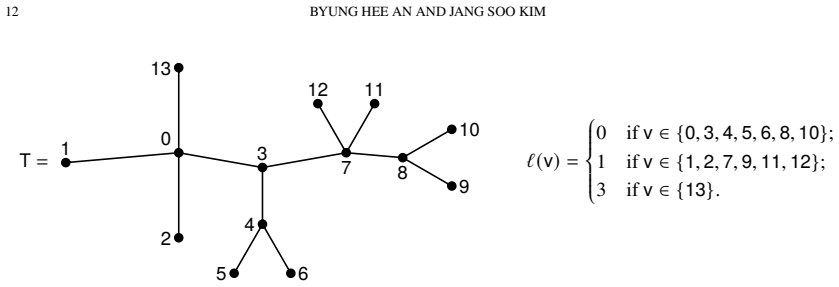
The central object is the binomial-convolution product $\ast$ of Eq. (2.1), which combines polynomials written in the binomial basis $\binom{k}{j}$ in such a way that the generating function of $(p_1\ast p_2)^+$ is the product of the generating functions of $p_1$ and $p_2$ (Lemma 2.2). This product is what assembles the local Hilbert polynomials across a one-bridge decomposition. The one-bridge decomposition formula, Corollary 3.11, $P^i_\Gamma(k)=\sum_{i_1+i_2=i}(P^{i_1}_{\Gamma_1}\ast P^{i_2}_{\Gamma_2})(k)$, is the step that upgrades 'eventually polynomial' to 'polynomial for all $k$', and it rests on the injectivity of the edge action $e\cdot(-)$ on homology (Proposition 3.10). The HE/SHE-configurations provide the combinatorial coefficients: each coefficient of $\binom{k}{j}$ counts standard configurations of $j$ dots and $i$ marked half edges obeying local rules at each essential vertex.
What would settle it
Compute $\dim_{\mathbb{F}} H_1(B_k\Gamma_{1,2})$ for the elementary bunch of grapes with one loop and two leaves for $k=0,1,2,3$ directly from the Świątkowski complex; if any value differs from $N_{1,2}(k)$ in Eq. (3.4), the residual polynomial is nonzero and Theorem 4.3 fails. More broadly, a single circumference-at-most-$1$ graph whose Betti number at some small $k$ disagrees with the claimed Hilbert polynomial would refute the paper's central claim.
Extended reading notes
Core claim
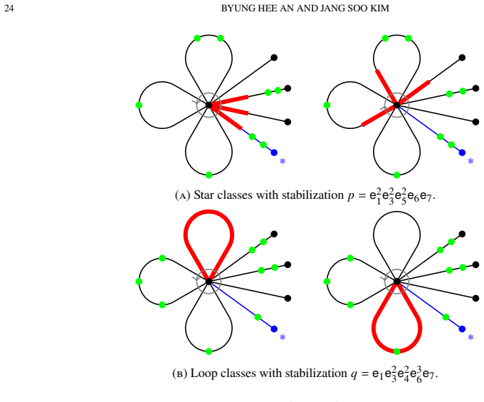
For any nontrivial bunch of grapes $\Gamma=(T,\ell)$, the residual polynomial $R_\Gamma(x,y)$ vanishes identically, so the Hilbert–Poincaré series of $B_\star\Gamma$ equals the generating series of its Hilbert polynomials exactly. Consequently, for each $i\ge 1$ and $k\ge 0$, $\dim_{\mathbb{F}} H_i(B_k\Gamma) = P^i_\Gamma(k) = \sum_{W\subseteq V_{\mathrm{ess}}(\Gamma),\, |W|=i} \big(\ast_{v\in W} P^1_{\Gamma_v}\big)(k)$, where $\ast$ is the binomial-convolution product defined in Eq. (2.1) and $\Gamma_v$ is the elementary local graph at the essential vertex $v$. The argument proceeds by induction on one-bridge decompositions along stem edges joining essential vertices, using injectivity of the edge-stabilization action to convert an eventual-polynomial statement into an exact one. A separate combinatorial model, the HE- and SHE-configurations, counts the coefficients of $P^i_\Gamma(k)$, and an explicit injective map realizes those configurations as homology cycles forming an $\mathbb{F}$-basis of $H_i(B_k\Gamma)$.
Load-bearing premise
The whole proof rests on the injectivity of the edge-stabilization action on the homology of every graph's configuration space, which is cited from the literature; if that map ever had a nontrivial kernel, torsion could appear and the exact one-bridge polynomial recurrence would break.
Editorial extensions
If this is right
- For every bunch of grapes, polynomiality of the $i$-th Betti number begins at $k=0$, so no stable-range threshold is needed for this family.
- The Hilbert polynomials $(P^i_\Gamma(k))_{i\ge0}$ determine the multiset of local data $\{(\ell(v),m(v))\}$ at essential vertices and vice versa; non-homeomorphic bunches of grapes with identical local data therefore have identical Betti-number polynomials.
- The coefficient formula turns the computation of $P^i_\Gamma(k)$ into a finite combinatorial count, giving all lower-order terms and not just the leading coefficient.
- Theorem 6.8 exhibits an explicit basis of $H_i(B_k\Gamma)$ indexed by HE-configurations, so every homology class is represented by star and loop classes supported near essential vertices with explicit stabilizations.
Reading between the lines
- If the injectivity of edge stabilization could be established or replaced by a resolution for graphs with multiple edges, the same binomial-convolution formalism might give exact polynomiality for graphs of circumference $2$, where the paper notes injectivity fails.
- The vanishing of the residual polynomial is equivalent to the absence of $\mathbb{F}[e]$-torsion in one-bridge decompositions; testing injectivity of $e\cdot(-)$ on other graph families could predict where exact polynomiality should hold.
- The SHE-configuration counts suggest a purely combinatorial algorithm for Betti numbers of graph configuration spaces that could be implemented and checked against known small-graph computations.
- Because the local data is recoverable from the whole polynomial sequence but not from the homeomorphism type, the Hilbert polynomials behave like a 'spectral' invariant of the graph's local geometry; it would be interesting to see whether a finite number of polynomials suffice for recognition.
Editorial analysis
A structured set of objections, weighed in public.
Referee Report
Summary. The paper studies unordered configuration spaces B_kΓ for graphs Γ whose topological circumference is at most one, called bunches of grapes. Its main theorem (Theorem 4.3) asserts that for every nontrivial bunch of grapes and every k≥0, the i-th Betti number of B_kΓ is given by a polynomial P_i^Γ(k), and it gives an explicit formula for this polynomial as a binomial-convolution product of the first Hilbert polynomials of the local graphs at the essential vertices; equivalently, the residual polynomial R_Γ(x,y) vanishes. Theorem 4.7 claims that the Hilbert polynomials determine the local data D(Γ). Section 5 gives a combinatorial interpretation of the b-coefficients of P_i^Γ(k) in terms of HE- and SHE-configurations, and Section 6 constructs homology classes from these configurations and claims that they form a basis of H_i(B_kΓ). The proof of Theorem 4.3 is an induction on the number of essential vertices, using the one-bridge decomposition (Corollary 3.11, Proposition 3.12) and the cited injectivity of edge stabilization from [ADCK19].
Significance. If Theorem 4.3 is correct, it resolves the onset of polynomiality for an entire family of graphs and gives explicit closed forms and coefficient counts, going well beyond the eventual polynomiality results of [ADCK20, ADCK22]. The proof is transparent and the combinatorial counts in Section 5 are explicit and essentially self-contained. The paper also correctly identifies the injectivity of edge stabilization as the precise input that upgrades eventual polynomiality to polynomiality for all k. However, the paper currently contains an overbroad statement in Theorem 4.7 and a major unproved claim in Theorem 6.8; these issues do not undermine the proof of Theorem 4.3 but do prevent acceptance in the present form.
major comments (2)
- [Section 4, Theorem 4.7] The 'if' direction of Theorem 4.7 is false as stated. Let Γ1 be an interval Γ_{0,2} and Γ2 a circle Γ_{1,0}; both lie in Grape and both have D(Γ)=∅, but by Proposition 3.8 we have P^1_{Γ1}(k)≡0 and P^1_{Γ2}(k)≡1. Thus D(Γ1)=D(Γ2) does not imply equality of Hilbert polynomials. The proof breaks down because it begins by defining d1=deg P^1_Γ, which is undefined when P^1_Γ=0. The theorem should either be restricted to nontrivial bunches of grapes or the no-essential-vertex case should be handled separately, for example by noting that within Grape the circle is distinguished from the interval by P^1.
- [Section 6.3, Theorem 6.8] After the construction of the map α:HE_i^Γ(k)→H_i(B_kΓ), the proof of Theorem 6.8 consists only of the sentence 'In summary, we obtain that the basis of the i-th homology group ... can be given by the set of HE-configurations.' No argument is supplied for injectivity or for the fact that the image spans H_i(B_kΓ). Since this claim is advertised as Theorem 1.4 in the introduction, this is a substantive gap. The authors should write out a proof—for example, an induction on essential vertices using Proposition 6.6 and the dimension formula of Theorem 4.3—or alternatively state the basis claim as a conjecture and remove it from the abstract.
minor comments (6)
- [Definition 5.1] In the definition of type-2 HE-configurations, the condition 'h=h2(e_r) for some 1<r≤ℓ+m' is ambiguous: for a non-loop edge e_r, the half edge h2(e_r) is not incident to the central vertex v. The intended meaning, confirmed by the count in Proposition 5.4, is that e_r is a loop; this should be stated explicitly.
- [Lemma A.1] The displayed identity '|SHE_{ℓ,0}(k)| binom(k,j)=|HE_{ℓ,0}(k)|' appears to be a typo; it should read |HE_{ℓ,0}(k)|=Σ_j |SHE_{ℓ,0}(j)| binom(k,j).
- [Appendix A, Proposition A.2] Proposition A.2 is stated with the comment 'we omit the proof.' Since this is still a claimed basis result, the authors should provide at least a brief justification, or state explicitly that it is a direct corollary of Proposition 6.6 with the modified SHE-definitions from Appendix A.
- [Section 5.2] The pivot edge for the root vertex v0 is not explicitly assigned; the text should state that e0 is the pivot edge of the local graph Γ_{v0}.
- [Remark 4.2] There is a typo: 'Considering Γ as a a topological space' should read 'Considering Γ as a topological space.'
- [Theorem 4.3 and Proposition 3.10] The proof of Theorem 4.3 relies on Proposition 3.10, cited from [ADCK19], and the paper does not reprove it. The authors are aware of the sharpness of this input (see the remark in Section 1.2), but it would be helpful to state explicitly in the statement of Theorem 4.3 that exact polynomiality for all k depends on that injectivity theorem.
Circularity Check
No circularity: the Hilbert-polynomial formula is proved by induction from external published theorems, not assumed or fitted.
full rationale
The central derivation is self-contained against prior independent results. Theorem 4.3 is proved by induction on the number of essential vertices: the base case (Proposition 3.8) uses the Ko-Park formula for first Betti numbers and [ADCK19] for vanishing of higher homology; the induction step uses the one-bridge decomposition theorem (Corollary 3.11 and Proposition 3.12). The only non-re-proved input is the injectivity of edge stabilization, [ADCK19, Prop. 5.21], which is a published theorem whose hypothesis (circumference-1 graphs) does not include the target equality, and which the paper explicitly notes fails for circumference-2 graphs. Section 5 gives an independent combinatorial count of HE-configurations matching the already-derived polynomial P^1_{Gamma_{ell,m}}(k); the coefficients are counted, not fitted. Theorem 6.8's basis statement is asserted after a short 'In summary' without a full injectivity/spanning proof, but it is an omitted proof rather than a circular step and is not needed for the main Hilbert-polynomial theorem. No equation reduces to its own input by construction.
Assumptions & free parameters
assumptions (6)
- domain assumption Edge stabilization e·(−) is injective on H_•(B★Γ) for every edge e (Prop. 3.10)
- domain assumption First Betti number of elementary bunch of grapes Γ_{ℓ,m} equals N_{ℓ,m}(k) (Eq. 3.5)
- domain assumption H_i(BΓ) is finitely generated over F[E] and eventually polynomial (Thm. 3.1, Cor. 3.2)
- standard math Homeomorphism invariance of configuration space homology under subdivision/smoothing of degree-2 vertices
- domain assumption Graphs of topological circumference at most 1 are exactly those obtained by attaching loops to a tree
- standard math F[e] is a PID and tensor products over it behave as in Cor. 3.11
Cite this review
Pith. "Pith review of Hilbert polynomials of configuration spaces over graphs of circumference at most 1." pith.science (2026). https://pith.science/paper/6IVJPI5O
@misc{pith2026250524416,
  author       = {Pith},
  title        = {Pith review of: Hilbert polynomials of configuration spaces over graphs of circumference at most 1},
  year         = {2026},
  howpublished = {\url{https://pith.science/paper/6IVJPI5O}},
  note         = {Machine review of arXiv:2505.24416}
}
abstract
The $ k $-configuration space $ B_k\Gamma $ of a topological space $ \Gamma $ is the space of sets of $ k $ distinct points in $ \Gamma $. In this paper, we consider the case where $ \Gamma $ is a graph of circumference at most $1$. We show that for all $ k\ge0 $, the $ i $-th Betti number of $ B_k\Gamma $ is given by a polynomial $P_\Gamma^i(k)$ in $ k $, called the Hilbert polynomial of $ \Gamma $. We find an expression for the Hilbert polynomial $P_\Gamma^i(k)$ in terms of those coming from the canonical $1$-bridge decomposition of $ \Gamma $. We also give a combinatorial description of the coefficients of $P_\Gamma^i(k)$.
Figures


Figures from the paper (11 more)




Reference graph
Works this paper leans on
-
[1]
Configuration spaces and braid groups of graphs
Aaron David Abrams. Configuration spaces and braid groups of graphs . ProQuest LLC, Ann Arbor, MI, 2000. Thesis (Ph.D.)--University of California, Berkeley
work page 2000
-
[2]
Drummond-Cole, and Ben Knudsen
Byung Hee An, Gabriel C. Drummond-Cole, and Ben Knudsen. Subdivisional spaces and graph braid groups. Doc. Math. , 24:1513--1583, 2019
work page 2019
-
[3]
Drummond-Cole, and Ben Knudsen
Byung Hee An, Gabriel C. Drummond-Cole, and Ben Knudsen. Edge stabilization in the homology of graph braid groups. Geom. Topol. , 24(1):421--469, 2020
work page 2020
-
[4]
Drummond-Cole, and Ben Knudsen
Byung Hee An, Gabriel C. Drummond-Cole, and Ben Knudsen. Asymptotic homology of graph braid groups. Geom. Topol. , 26(4):1745--1771, 2022
work page 2022
-
[5]
On the second homology of planar graph braid groups
Byung Hee An and Ben Knudsen. On the second homology of planar graph braid groups. J. Topol. , 15(2):666--691, 2022
work page 2022
-
[6]
Betti numbers of unordered configuration spaces of small graphs
Gabriel C. Drummond-Cole. Betti numbers of unordered configuration spaces of small graphs. arXiv:1906.00692, 2020
work page Pith review arXiv 1906
-
[7]
Discrete M orse theory and graph braid groups
Daniel Farley and Lucas Sabalka. Discrete M orse theory and graph braid groups. Algebr. Geom. Topol. , 5:1075--1109, 2005
work page 2005
-
[8]
On the cohomology rings of tree braid groups
Daniel Farley and Lucas Sabalka. On the cohomology rings of tree braid groups. J. Pure Appl. Algebra , 212(1):53--71, 2008
work page 2008
Show all 13 references
-
[9]
Configuration spaces and braid groups on graphs in robotics
Robert Ghrist. Configuration spaces and braid groups on graphs in robotics. In Knots, braids, and mapping class groups---papers dedicated to J oan S . B irman ( N ew Y ork, 1998) , volume 24 of AMS/IP Stud. Adv. Math. , pages 29--40. Amer. Math. Soc., Providence, RI, 2001
1998
-
[10]
Graph braid groups and right-angled A rtin groups
Jee Hyoun Kim, Ki Hyoung Ko, and Hyo Won Park. Graph braid groups and right-angled A rtin groups. Trans. Amer. Math. Soc. , 364(1):309--360, 2012
2012
-
[11]
Graph 4-braid groups and M assey products
Ki Hyoung Ko, Joon Hyun La, and Hyo Won Park. Graph 4-braid groups and M assey products. Topology Appl. , 197:133--153, 2016
2016
-
[12]
Characteristics of graph braid groups
Ki Hyoung Ko and Hyo Won Park. Characteristics of graph braid groups. Discrete Comput. Geom. , 48(4):915--963, 2012
2012
-
[13]
On rigidity and the isomorphism problem for tree braid groups
Lucas Sabalka. On rigidity and the isomorphism problem for tree braid groups. Groups Geom. Dyn. , 3(3):469--523, 2009
2009
Reviewed August 7, 2026 · model on record in the stance chip above.
Discussion (0). Sign in to comment.