Continuous Fourier Transform: A practical approach for truncated signals and suggestions for improvements in thermography
Pith reviewed 2026-05-25 10:52 UTC · model grok-4.3
The pith
Polynomial fitting to the start of cooling curves lets the continuous Fourier transform deliver consistent amplitude and phase without artifacts for pulse phase thermography.
A machine-rendered reading of the paper's core claim, the machinery that carries it, and where it could break.
Core claim
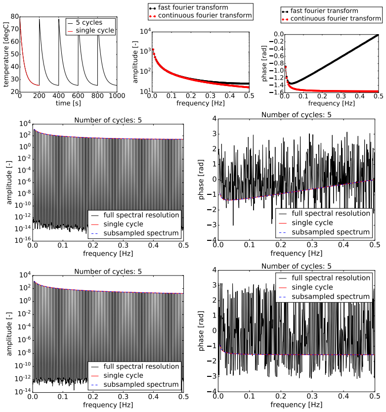
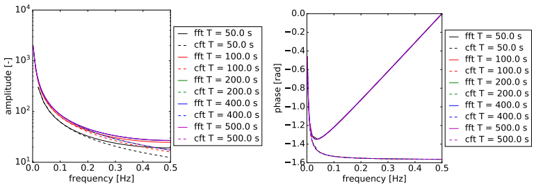
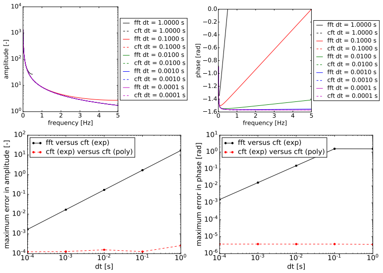
The proposed polynomial-fitting continuous Fourier transform method produces consistent amplitude and phase with no artifacts for cooling curves in pulse phase thermography, unlike existing fast Fourier transform methods which depend on sampling rates and introduce inconsistencies, provided the start of the cooling curves is sufficiently represented.
What carries the argument
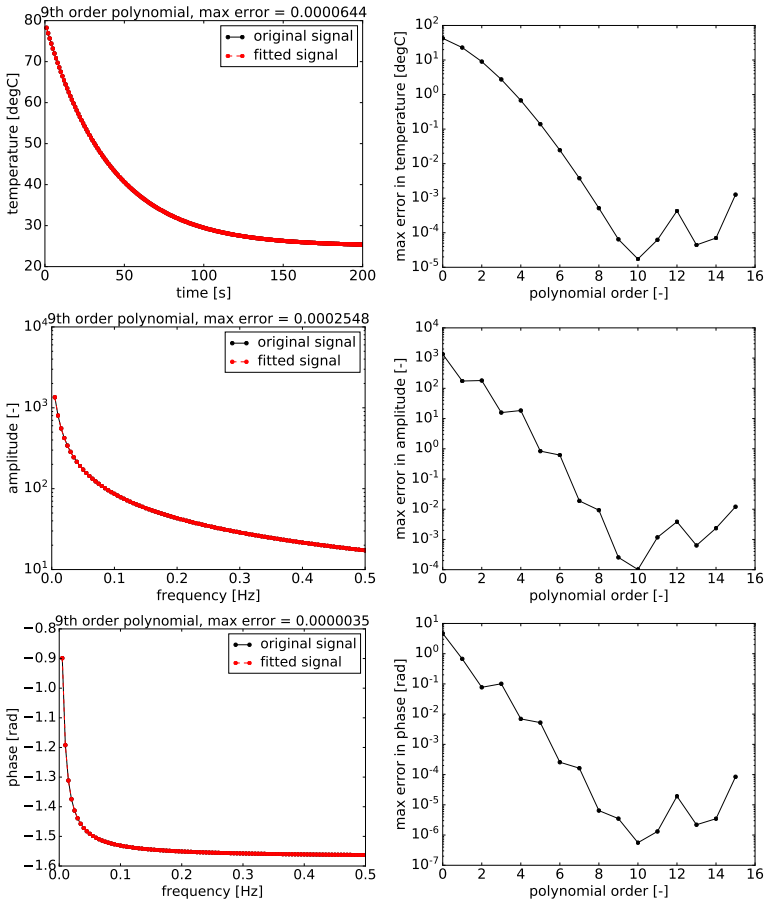
Polynomial fit to the early portion of the cooling curve, which allows the continuous Fourier transform to be applied to truncated signals without truncation-induced errors.
If this is right
- Existing FFT methods in PPT depend on sampling rates and produce artifacts in amplitude and phase for decay curves.
- The polynomial CFT method avoids these artifacts and gives consistent results when the curve start is well sampled.
- Consistent amplitude and phase support better defect identification in NDT.
- Standardized methods could enable unified datasets for machine learning in thermography.
Where Pith is reading between the lines
- Applying this to other fields with truncated exponential decays could reduce analysis inconsistencies.
- Integration with automated systems might improve defect recognition accuracy in industrial NDT.
- The analytical benchmarks for CFT on truncated signals could serve as a general reference for signal processing of finite-duration data.
Load-bearing premise
A polynomial fit to the early portion of the cooling curve accurately captures the underlying signal behavior required for the CFT to match the true decay.
What would settle it
A direct comparison on synthetic cooling curves with known exact Fourier transforms, checking if the polynomial CFT matches the analytical result when the start is included but diverges otherwise.
Figures
read the original abstract
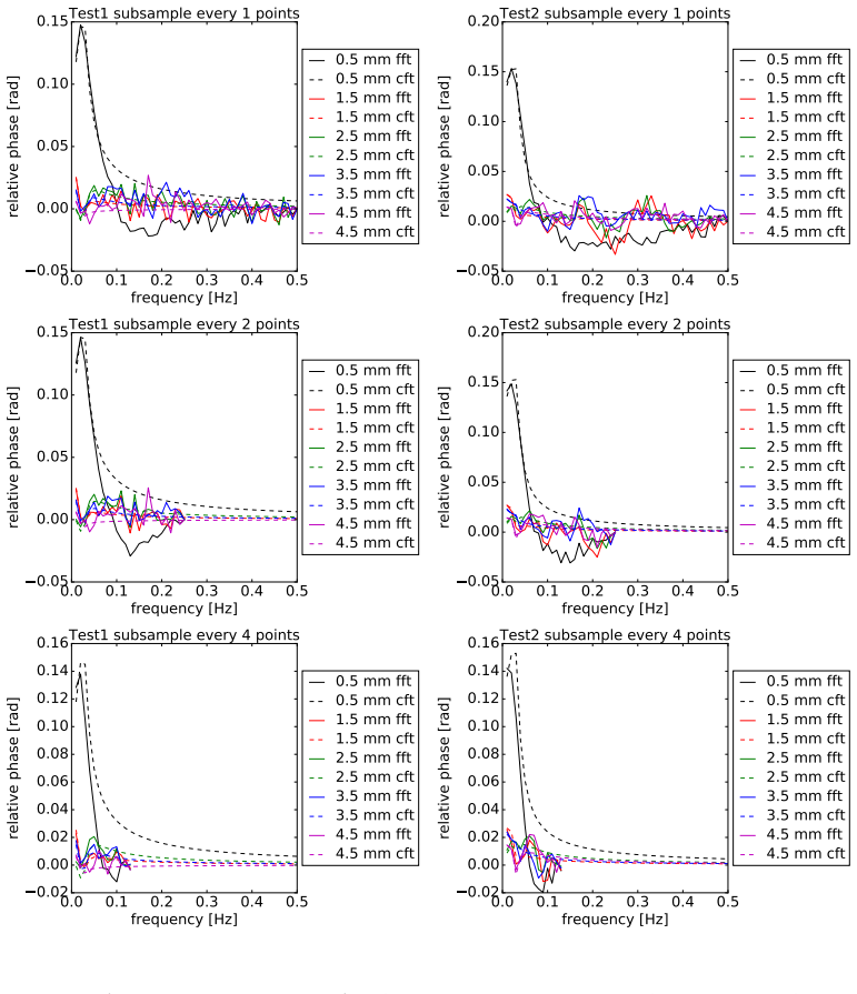
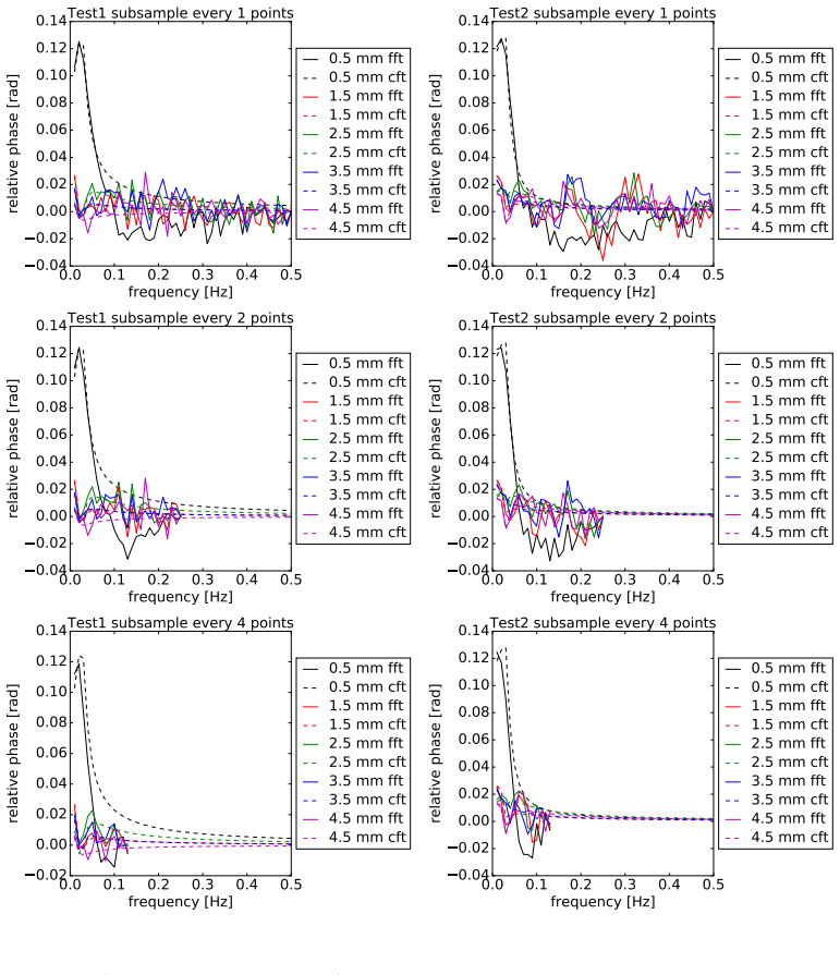
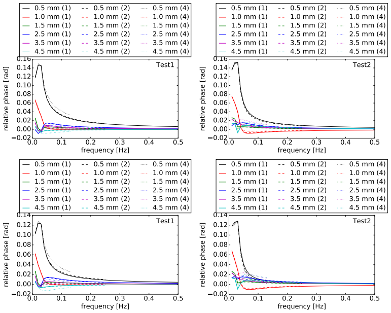
The fundamentals of Fourier Transform are presented, with analytical solutions derived for Continuous Fourier Transform (CFT) of truncated signals, to benchmark against Fast Fourier Transform (FFT). Certain artifacts from FFT were identified for decay curves. An existing method for Infrared Thermography, Pulse Phase Thermography (PPT), was benchmarked against a proposed method using polynomial fitting with CFT, to analyse cooling curves for defect identification in Non-Destructive Testing (NDT). Existing FFT methods used in PPT were shown to be dependent on sampling rates, with inherent artifacts and inconsistencies in both amplitude and phase. It was shown that the proposed method produced consistent amplitude and phase, with no artifacts, as long as the start of the cooling curves are sufficiently represented. It is hoped that a collaborative approach will be adopted to unify data in Thermography for machine learning models to thrive, in order to facilitate automated geometry and defect recognition and move the field forward.
Editorial analysis
A structured set of objections, weighed in public.
Referee Report
Summary. The paper presents fundamentals of the Fourier Transform and derives analytical solutions for the Continuous Fourier Transform (CFT) of truncated signals to benchmark against the Fast Fourier Transform (FFT). It identifies sampling-rate dependent artifacts and inconsistencies in amplitude and phase when using FFT within Pulse Phase Thermography (PPT) for cooling-curve analysis in infrared thermography for non-destructive testing. The authors propose a polynomial-fitting approach combined with CFT that is claimed to yield consistent amplitude and phase with no artifacts, provided the start of the cooling curves is sufficiently represented. The work concludes with a call for unified thermography datasets to support machine-learning applications in defect recognition.
Significance. If the central claim holds, the polynomial-fitting CFT method could offer a practical improvement over FFT-based PPT by removing truncation artifacts in thermographic NDT, and the data-unification suggestion could aid reproducibility for ML models. The derivation of analytical CFT solutions for truncated signals is a potential strength if they are fully presented and used for validation.
major comments (2)
- [Abstract] Abstract: the central claim that the proposed method 'produced consistent amplitude and phase, with no artifacts' depends on the untested premise that a polynomial fit to the initial segment of a cooling curve reproduces the frequency content of the underlying truncated diffusive decay. No explicit error bound, truncation-error analysis, or direct comparison of the polynomial-fitted CFT against the paper's own analytical CFT solutions for known truncated exponentials is referenced.
- [Abstract] Abstract: the qualifier 'as long as the start of the cooling curves are sufficiently represented' is not accompanied by a quantitative criterion (e.g., number of points, time window relative to the thermal diffusion time, or residual threshold) nor by a sensitivity study on polynomial degree, leaving the method with free parameters whose effect on amplitude/phase consistency is unexamined.
Simulated Author's Rebuttal
We thank the referee for the constructive comments on our manuscript. The points raised identify areas where additional validation would strengthen the presentation of the polynomial-fitting CFT method. We agree that revisions are warranted and outline our responses below.
read point-by-point responses
-
Referee: [Abstract] Abstract: the central claim that the proposed method 'produced consistent amplitude and phase, with no artifacts' depends on the untested premise that a polynomial fit to the initial segment of a cooling curve reproduces the frequency content of the underlying truncated diffusive decay. No explicit error bound, truncation-error analysis, or direct comparison of the polynomial-fitted CFT against the paper's own analytical CFT solutions for known truncated exponentials is referenced.
Authors: We agree that the manuscript would benefit from an explicit comparison of the polynomial-fitted CFT results against the analytical CFT solutions derived earlier in the paper for truncated signals. The current work shows empirical consistency of amplitude and phase across sampling rates but does not include this direct benchmark or associated error analysis for the fitted cooling curves. We will add a dedicated validation subsection with such comparisons and truncation-error bounds in the revised manuscript. revision: yes
-
Referee: [Abstract] Abstract: the qualifier 'as long as the start of the cooling curves are sufficiently represented' is not accompanied by a quantitative criterion (e.g., number of points, time window relative to the thermal diffusion time, or residual threshold) nor by a sensitivity study on polynomial degree, leaving the method with free parameters whose effect on amplitude/phase consistency is unexamined.
Authors: We acknowledge that the condition is stated qualitatively without supporting quantitative guidance or sensitivity analysis. In revision we will define a concrete criterion (for example, requiring the captured initial segment to span at least a specified multiple of the characteristic thermal diffusion time, together with a fit-residual threshold) and will include a sensitivity study examining the effect of polynomial degree on the resulting amplitude and phase values. revision: yes
Circularity Check
No circularity: analytical CFT derivation and polynomial approximation remain independent of fitted outputs
full rationale
The paper first derives closed-form CFT expressions for truncated signals (to benchmark FFT artifacts), then applies a separate polynomial fit to early cooling data before computing CFT. Neither step reduces by the paper's own equations to a parameter that is fitted and then relabeled as a prediction; the consistency claim follows from direct comparison on data rather than from self-definition or self-citation load-bearing. The polynomial step is an explicit modeling choice whose validity is external to the derivation itself. No uniqueness theorem, ansatz smuggling, or renaming of known results is invoked in a load-bearing way.
Axiom & Free-Parameter Ledger
free parameters (1)
- polynomial degree or coefficients
axioms (2)
- standard math Standard properties of the continuous Fourier transform hold for the truncated signals under consideration.
- domain assumption Cooling curves in thermography can be adequately represented by a polynomial fit over the recorded interval.
Reference graph
Works this paper leans on
-
[1]
Fourier transform, http://mathworld.wolfram.com/ FourierTransform.html, (accessed June 18, 2019)
work page 2019
-
[2]
X. Maldague, S. Marinetti, Pulse phase infrared thermography, Journal of Applied Physics 79 (1996) 2694–2698
work page 1996
-
[3]
F. Galmiche, M. Leclerc, X. P. Maldague, Time aliasing problem in pulsed-phased thermography, in: Thermosense XXIII, volume 4360, International Society for Optics and Photonics, 2001, pp. 550–554
work page 2001
-
[4]
C. Ibarra-Castanedo, X. Maldague, Review of pulsed phase thermogra- phy, in: Thermosense: Thermal Infrared Applications XXXVII, volume 9485, International Society for Optics and Photonics, 2015, p. 94850T
work page 2015
-
[5]
C. Ibarra Castanedo, Quantitative subsurface defect evaluation by pulsed phase thermography: depth retrieval with the phase (2005)
work page 2005
-
[6]
C. Ibarra-Castanedo, X. Maldague, Pulsed phase thermography re- viewed, Quantitative Infrared Thermography Journal 1 (2004) 47–70
work page 2004
-
[7]
Z. Wang, G. Tian, M. Meo, F. Ciampa, Image processing based quanti- tative damage evaluation in composites with long pulse thermography, NDT & E International 99 (2018) 93–104. 14
work page 2018
-
[8]
E. DAccardi, F. Palano, R. Tamborrino, D. Palumbo, A. Tat` ı, R. Terzi, U. Galietti, Pulsed phase thermography approach for the characteriza- tion of delaminations in cfrp and comparison to phased array ultrasonic testing, Journal of Nondestructive Evaluation 38 (2019) 20
work page 2019
- [9]
-
[10]
M. Ishikawa, M. Ando, M. Koyama, H. Nishino, Active thermographic inspection of carbon fiber reinforced plastic laminates using laser scan- ning heating, Composite Structures 209 (2019) 515–522
work page 2019
- [11]
-
[12]
X. Tian, M. Y. Yin, K. H. H. Goh, Identifying the geometry of an object using lock-in thermography, arXiv preprint arXiv:1903.02854 (2019)
work page internal anchor Pith review Pith/arXiv arXiv 1903
-
[13]
K. Goh, Q. Lim, P. Pallathadka, Asynchronous lock in thermography of 3d printed pla and abs samples, arXiv preprint arXiv:1805.01343 (2018)
work page internal anchor Pith review Pith/arXiv arXiv 2018
-
[14]
M. H. Wong, K. H. H. Goh, Infrared thermography of complex 3d printed components, arXiv preprint arXiv:1810.05413 (2018). 15 Table 1: Sample tolerance values for polynomial fit of a certain order, for 13 sample points Tolerance 5th order 7th order 9th order 11th order Intensity (max) [-] 600 300 150 90 Intensity (mean) [-] 90 40 20 12 Temperature (max) [K]...
work page internal anchor Pith review Pith/arXiv arXiv 2018
discussion (0)
Sign in with ORCID, Apple, or X to comment. Anyone can read and Pith papers without signing in.