REVIEW 4 major objections 6 minor 49 references
Statistical modeling of groundwater quality assessment in Iran using a flexible Poisson likelihood
T0 review · 4 major / 6 minor · reviewed 2026-08-14 · deepseek-v4-flash
Pith's one-line read A Bayesian gamma-count model with the SPDE approximation improves spatial count predictions over Poisson and negative binomial alternatives.
desk verdict Spatial gamma-count regression is a natural and useful extension; the evidence for its superiority is currently undercut by a misread test statistic and a broken negative binomial baseline. read the letter →
The pith
A machine-rendered reading of the paper's core claim, the machinery that carries it, and where it could break.
The reading
What carries the argument
The central object is the gamma-count distribution from renewal theory: replace the exponential waiting times that generate the Poisson distribution by gamma waiting times $\tau_k\sim\operatorname{Gamma}(\alpha,\gamma)$. The count in $(0,T)$ then has probability mass function as the difference of two incomplete gamma CDFs, and the gamma's reproductive property keeps this a stable numerical expression. The dispersion parameter $\alpha$ is the single additional ingredient: it collapses the model to Poisson at $\alpha=1$, and indexes over- and under-dispersion through negative and positive duration dependence. The spatial machinery is the SPDE representation of a Matern Gaussian field as a Gaussian Markov random field, which gives a sparse precision matrix; combined with the latent-Gaussian structure, this is what makes INLA fast enough for routine use.
What would settle it
Take spatial count data with strong over-dispersion in one half of the domain and near-Poisson behavior in the other, fit the proposed constant-$\alpha$ gamma-count model, and compare its coverage and WAIC with a model that lets $\alpha$ vary spatially. If the flexible-$\alpha$ model is clearly better, the central practical claim fails for spatially heterogeneous dispersion.
Extended reading notes
Core claim
The paper's central claim is that a gamma-count likelihood coupled with a Gaussian spatial random field is a better sampling model for spatially referenced dispersed counts than the usual Poisson and negative binomial alternatives. In the gamma-count construction, waiting times are iid $\operatorname{Gamma}(\alpha,\gamma)$, and the count pmf is $P(Y=y)=G(y\alpha,\gamma T)-G((y+1)\alpha,\gamma T)$, where $G$ is the incomplete gamma ratio; $\alpha=1$ gives Poisson, $\alpha<1$ over-dispersion, and $\alpha>1$ under-dispersion. Writing $\gamma_i=\alpha\exp(x_i'\beta+\varphi(s_i))$ keeps the model inside the latent-Gaussian class, so INLA computes posterior marginals without MCMC. For the groundwater data the estimated dispersion is $\hat{\alpha}=0.309$, and WAIC, DIC, and cross-validated logarithmic score all prefer the gamma-count model over Poisson and negative binomial.
Load-bearing premise
The load-bearing premise is that a single dispersion parameter $\alpha$ describes every location and observation; if dispersion varies spatially, the gamma-count likelihood is misspecified and the reported gains may not transfer.
Editorial extensions
If this is right
- Any count dataset currently forced into a Poisson or negative binomial model can be re-fit with the gamma-count likelihood through INLA, with the Poisson result recovered at $\alpha=1$.
- Spatial predictions of the response field inherit the improved dispersion modeling; in the Golestan example the estimated range is smoother, about 64 km, and identifies low-quality water in the central region.
- Simulation results in the paper indicate the gamma-count model recovers regression and Matern covariance parameters with lower RMSE than Poisson and negative binomial under both over- and under-dispersion, so inference about covariate effects is more reliable in those settings.
- Because the gamma-count family nests the Poisson model, model comparison via WAIC and DIC gives a direct check for whether the extra dispersion parameter is needed.
Reading between the lines
- Editorial inference: letting $\log\alpha$ depend on covariates or on a second spatial field is the natural next step; if dispersion varies by region, the constant-$\alpha$ model would understate uncertainty in high-dispersion areas.
- The same renewal-theory construction with Weibull or lognormal waiting times should transfer directly to the INLA-SPDE machinery, giving a family of flexible spatial count models rather than a single one.
- A likely unstated payoff is that the gamma-count likelihood should also work for spatio-temporal counts and point-pattern aggregation, where over- and under-dispersion are common; the paper's arguments do not depend on the groundwater setting.
Signed reviews
Editorial analysis
A structured set of objections, weighed in public.
Referee Report
Summary. The paper proposes a Bayesian hierarchical spatial gamma-count (GC) regression model for count data, built on the renewal-theoretic idea that nonexponential waiting times induce a flexible count distribution capable of capturing both over- and under-dispersion. The authors embed this GC likelihood in a latent Gaussian model and fit it with INLA and the SPDE approach for geostatistical data. They apply the model to a groundwater-quality dataset from Golestan Province, Iran, where the response is the number of months (out of the study period) in which electrical conductivity indicates drinkable water. The paper claims, on the basis of a simulation study and the real-data example, that the GC model significantly outperforms both Poisson and negative binomial alternatives. The manuscript also reports model-selection criteria (WAIC, DIC, log score) and posterior summaries for regression and spatial parameters.
Significance. If the central claim is correct, the paper offers practitioners a useful and computationally tractable extension of spatial count models: a single additional dispersion parameter that nests the Poisson model, implemented through R-INLA. This would be a practical contribution to spatial epidemiology and environmental statistics. The paper also demonstrates the use of the already-implemented 'gammacount' family in R-INLA, and the reliance on the SPDE approach is standard. However, the current manuscript contains several internal errors and an apparently broken negative binomial baseline in the simulations, so the strength of the evidence for the headline claim is not yet established.
major comments (4)
- [Section 1.2, Eq. (1)] The Dean-Lawless test statistic is reported as T = -5.4466. Because the test in Eq. (1) is a one-sided test of H0: tau = 0 versus H1: tau > 0, a large negative value indicates underdispersion, not overdispersion. The text then states that H0 is rejected at level 0.05 and concludes that the counts are overdispersed. This is logically inconsistent. Moreover, Section 5 reports an estimated dispersion parameter alpha = 0.309 with 95% credible interval (0.203, 0.434), which by the paper's own convention (alpha < 1) implies overdispersion, contradicting the implication of the test statistic. Please correct the sign interpretation or the test computation, and reconcile the contradictory conclusions.
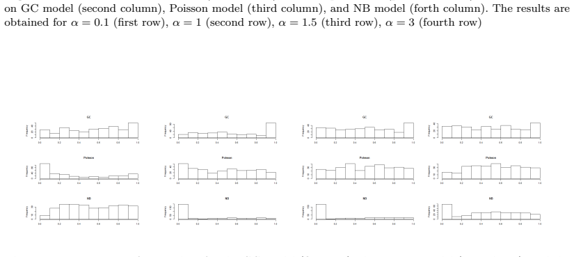
- [Section 4, Table 1] The negative binomial baseline in the simulation appears to be non-converged or incorrectly implemented. When alpha = 1 (the true model is Poisson), the NB model yields RMSEs of 20.1498 for the intercept and 5.6965 for the slope, while the Poisson and GC models have RMSEs around 0.22 and 0.06. Since the NB model nests the Poisson model, a correctly specified and well-fitted NB should have RMSEs comparable to those of the Poisson model. The large RMSEs indicate a convergence failure or a faulty parameterization of the NB model in R-INLA. Consequently, the claim of a 'significant improvement over the negative binomial' model based on this simulation study is not supported by the presented evidence. The simulations should be rerun with a reliably fitted NB baseline, and the results should be reported alongside a discussion of any encountered convergence issues.
- [Section 5, after Table 5] The PC priors for the Matérn field parameters are set using estimates obtained from the same dataset. The authors first fit the selected model and obtain estimates sigma = 0.74 and r = 49.18, and then use these estimates to specify P(sigma > 0.74) = 0.05 and P(r < 49) = 0.05. This is a double use of the data: the data are used to choose the prior hyperparameters and then used again to obtain the posterior. This empirical-Bayes-like procedure should be explicitly acknowledged and justified, or the priors should be fixed a priori. As written, the posterior credible intervals in Table 6 do not account for this prior adaptation and may be overconfident.
- [Section 5, Table 5] The WAIC values in Table 5 range from 652.540 to 18336.51, while the DIC values range from 221.052 to 236.823. WAIC and DIC are both information criteria typically reported on the same deviance scale, and such a discrepancy of two orders of magnitude is implausible. This suggests that the WAIC (or DIC) computation is incorrect or that the criteria are defined on different scales without clarification. Since the model-selection conclusions rely on these criteria, please verify the computational definition, check the implementation, and report the criteria on a consistent scale.
minor comments (6)
- [Throughout] The manuscript contains many typesetting errors, including garbled characters (e.g., 'flexible' for 'flexible', 'shuch' for 'such', 'T able' for 'Table'), inconsistent spacing, and missing article template formatting. A careful editorial pass is needed.
- [References, item [28]] The reference to Pearson (1894) is listed with the year '1994' in the reference list. The correct year is 1894.
- [Section 2, Eq. (4)] The infinite sum in Eq. (4) is stated to have no closed form; please clarify what numerical method is used to evaluate it in the likelihood computations, as this affects the reproducibility of the results.
- [Section 3, Eq. (9) and following text] The definitions of the SPDE precision-matrix components ilde{C} and G are given in prose; it would be clearer to define them with explicit equations, especially the diagonal matrix ilde{C}.
- [Section 4, Table 3] The text says MSPE is computed for 'one simulated GRF' but Table 3 appears to report averages over replications. Please clarify how MSPE is aggregated across the simulation replications.
- [Section 5, Figure 6] The prediction maps in Figure 6 are described only briefly; a sentence explaining what the color scale represents and how the standard deviation maps should be interpreted would improve readability.
Circularity Check
No circularity: the gamma-count likelihood and the INLA/SPDE implementation are not defined in terms of the quantities the paper claims to predict.
full rationale
The paper's central claim is that a spatial gamma-count model improves on Poisson and negative binomial alternatives. The gamma-count pmf (Eq. 2) is derived from gamma waiting times via renewal theory, independent of the groundwater data; the regression model (Eq. 8) links the predictor to E(τ) and nests Poisson at α=1. The simulation study draws data from the assumed GC model, so it is a generative consistency check rather than a tautological proof. The real-data analysis uses fixed likelihoods and standard SPDE/INLA machinery; no fitted parameter is renamed as a prediction. The empirical-Bayes step in Section 5 — using first-stage estimates σ̂=0.74 and r̂=49.18 to set PC-prior quantiles (P(σ>0.74)=0.05, P(r<49)=0.05) and then refitting the same data — double-uses the data and is a legitimate statistical concern, but it does not make the WAIC/DIC comparison equivalent to those estimates by construction; the posterior range actually moves away from the prior constraint (r posterior mean 64.46 km vs prior r<49 km). Self-citations to INLA/SPDE/PC-prior literature are methodological and not load-bearing in the model derivation. The reported Dean-Lawless statistic T=-5.45 appears inconsistent with the claimed overdispersion conclusion, but that is a correctness/evidence issue, not circularity. Under the stated rules, no specific equation-level or definitional reduction is exhibited, so the appropriate circularity score is 0.
Assumptions & free parameters
free parameters (5)
- alpha (gamma shape / dispersion) =
0.309 posterior mean in application; simulation settings 0.1, 1, 1.5, 3
- sigma (marginal SD of Matérn field) =
Posterior mean about 0.74 in application
- r (spatial range) =
Posterior mean 49 km in preliminary fit; 64.46 km in final GC model
- PC prior hyperparameters sigma0, r0 =
sigma0=0.74, r0=49
- Prior hyperparameters a, b, Sigma_beta, c, d, e, f =
a=0.01, b=0.01, Sigma_beta=1000I, c=log(0.02), d=10, e=log(14), f=10
assumptions (6)
- domain assumption Waiting times between events are i.i.d. Gamma(alpha, gamma).
- domain assumption Counts are conditionally independent given the latent spatial field and parameters.
- domain assumption The spatial effect follows a stationary isotropic Matérn GRF with smoothness nu=1, approximated by SPDE.
- domain assumption The gamma-count likelihood can be treated as a latent Gaussian model family in R-INLA with linear predictor entering as gamma = alpha exp(eta).
- domain assumption Constant dispersion alpha across all observations.
- domain assumption PC priors for Matérn parameters are appropriate.
Cite this review
Pith. "Pith review of Statistical modeling of groundwater quality assessment in Iran using a flexible Poisson likelihood." pith.science (2026). https://pith.science/paper/6LQPLYUP
@misc{pith2026190802344,
  author       = {Pith},
  title        = {Pith review of: Statistical modeling of groundwater quality assessment in Iran using a flexible Poisson likelihood},
  year         = {2026},
  howpublished = {\url{https://pith.science/paper/6LQPLYUP}},
  note         = {Machine review of arXiv:1908.02344}
}
read the original abstract
Assessing water quality and recognizing its associated risks to human health and the broader environment is undoubtedly essential. Groundwater is widely used to supply water for drinking, industry, and agriculture purposes. The groundwater quality measurements vary for different climates and various human behaviors, and consequently, their spatial variability can be substantial. In this paper, we aim to analyze a groundwater dataset from the Golestan province, Iran, for November 2003 to November 2013. Our target response variable to monitor the quality of groundwater is the number of counts that the quality of water is good for a drink. Hence, we are facing spatial count data. Due to the ubiquity of over or underdispersion in count data, we propose a Bayesian hierarchical modeling approach based on the renewal theory that relates nonexponential waiting times between events and the distribution of the counts, relaxing the assumption of equidispersion at the cost of an additional parameter. Particularly, we extend the methodology for the analysis of spatial count data based on the gamma distribution assumption for waiting times. The model can be formulated as a latent Gaussian model, and therefore, we can carry out the fast computation by using the integrated nested Laplace approximation method. The analysis of the groundwater dataset and a simulation study show a significant improvement over both Poisson and negative binomial models.
Figures


Figures from the paper (4 more)


Reference graph
Works this paper leans on
- [1]
-
[2]
Bear, Hydraulics of groundwater, NewYork: Courier Corporation, 1979
J. Bear, Hydraulics of groundwater, NewYork: Courier Corporation, 1979
work page 1979
-
[3]
M. Blangiardo, M. Cameletti, G. Baioc, and H. Rue, Spatial and spatio-temporal models with R-INLA, Spatial and Spatio-temporal Epidemiology 7 (2013), pp. 39–55
work page 2013
-
[4]
N. Breslow and D. G. Clayton, Approximate inference in generalized linear mixed models, Journal of the American Statistical Association 88 (1993), pp. 9–25
work page 1993
-
[5]
A. C. Cameron and P. K. Trivedi, Regression Analysis of Count Data , Second Eddition, New York: Cambridge University Press, 2013
work page 2013
-
[6]
J. Cotruvo, J. K. Fawell, M. Giddings, P. Jackson, Y. Magara, A.V. Festo Ngowi, and E. Ohanian, Background document for development of WHO guidelines for drinking-water quality , 2011. URL https : //www.who.int/water sanitationhealth/dwq/chemicals/hardness.pdf
work page 2011
-
[7]
D. R. Cox, Renewal Theory, Methuen, London, 1962
work page 1962
-
[8]
Cressie, Statistics for Spatial Data , John Wiley and Sons, Inc, 1993
N. Cressie, Statistics for Spatial Data , John Wiley and Sons, Inc, 1993
work page 1993
Show all 49 references
-
[9]
Dawid, Statistical theory: The prequential approach , Journal of the Royal Statistical Society, Series A, 147 (1984), pp
A. Dawid, Statistical theory: The prequential approach , Journal of the Royal Statistical Society, Series A, 147 (1984), pp. 278–292
1984
-
[10]
Dean and J
C. Dean and J. F. Lawless, Tests for detecting overdispersion in Poisson regression models, Journal of the American Statistical Association 84 (1989), pp. 467–472
1989
-
[11]
Fahrmeir and G
L. Fahrmeir and G. Tutz, Multivariate Statistical Modelling Based on Generalized Linear Models, 2nd ed., New York: Springer, 2001
2001
-
[12]
Fuglstad, D
G. Fuglstad, D. Simpson, F. Lingren, and H. Rue, Constructing priors that penalize the complexity of Gaussian random fields , Journal of the American Statistical Association, 114 (2019), pp. 445–452
2019
-
[13]
Gelman, J
A. Gelman, J. Hwang, and A. Vehtari, Understanding predictive information criteria for Bayesian models, Statistics and Computing, 24 (2014), pp. 997–1016
2014
-
[14]
Gonzales-Barron and F
U. Gonzales-Barron and F. Butler, Characterisation of within-batch and between-batch variability in microbial counts in foods using Poisson-gamma and Poisson-lognormal re- gression models, Food Control 22 (2011), pp. 1268–1278
2011
-
[15]
G. M. Hornberger, P. L. Wiberg, J. P. Raffensperger, and P. D’Odorico, Elements of Physical Hydrology, JHU Press, 2014
2014
-
[16]
E. T. Krainski, V. G´ omez-Rubio, H. Bakka, A. Lenzi, D. Castro-Camilo, D. Simpson, F. Lindgren, and H. Rue, Advanced Spatial Modeling with Stochastic Partial Differential Equations Using R and INLA , New York: Chapman and Hall/CRC, 2018
2018
-
[17]
Lewis, Small Dams , CRC Press/Balkema, 2003
B. Lewis, Small Dams , CRC Press/Balkema, 2003
2003
-
[18]
Lindgren, Continuous domain spatial models in R-INLA , The ISBA Bulletin 19 (2012, december), URL: http://www.r-inla.org/examples/tutorials/spde-from-the-isba-bulletin
F. Lindgren, Continuous domain spatial models in R-INLA , The ISBA Bulletin 19 (2012, december), URL: http://www.r-inla.org/examples/tutorials/spde-from-the-isba-bulletin
2012
-
[19]
Lindgren, H
F. Lindgren, H. Rue, and J. Lindstrom, An explicit link between Gaussian fields and Gaus- sian Markov random fields: the stochastic partial differential equation approach , Journal of the Royal Statistical Society, Series B, 73 (2011), pp. 423–498
2011
-
[20]
D. Lord, S. R. Geedipally, and S. D. Guikema, Extension of the application of Conway- Maxwell-Poisson models: analyzing traffic crash data exhibiting underdispersion , Risk Analysis: An Official Publication of the Society for Risk Analysis 30 (2010), pp. 1268– 1276
2010
-
[21]
D. Lord, S. D. Guikema, and S. R. Geedipally, Application of the Conway-Maxwell- Pois- son generalized linear model for analyzing motor vehicle crashes , Accident; Analysis and Prevention 40 (2008), pp. 1123–1134
2008
-
[22]
T. G. Martins, D. Simpson, F. Lindgren, and H. Rue, Bayesian computing with INLA: new features, Computational Statistics and Data Analysis 67 (2013), pp. 68–83
2013
-
[23]
McShane, M
B. McShane, M. Adrian, E. T. Bradlow, and P. S. Fader, Count models based on Weibull interarrival times, Journal of Business and Economic Statistics 26 (2008), pp. 369–378
2008
-
[24]
J. A. Nelder and R. W. M. Wedderburn, Generalized linear models, Journal of the Royal Statistical Society, Series A, 135 (1972), pp. 370–384
1972
-
[25]
S. Muff, A. Riebler, L. Held, H. Rue, and P. Saner,Bayesian analysis of measurement error models using integrated nested Laplace approximations , Journal of the Royal Statistical Society, Series C (Applied Statistics) 64 (2015), pp. 231–252. 22
2015
-
[26]
S. H. Ong, A. Biswas, S. Peiris, and Y. C. Low, Count distribution for generalized Weibull duration with applications, Communications in Statistics-Theory and Methods 44 (2015), pp. 4203-4216
2015
-
[27]
M. Paul, A. Riebler, L. M. Bachmann, H. Rue, and L. Held, Bayesian bivariate meta- analysis of diagnostic test studies using integrated nested Laplace approximations , Statis- tics in Medicine, 29 (2010), pp. 1325–1339
2010
-
[28]
Pearson, Contributions to the theory of mathematical evolution , Philosiphcal Transi- tions of the Royal society of London 185 (1994), pp
K. Pearson, Contributions to the theory of mathematical evolution , Philosiphcal Transi- tions of the Royal society of London 185 (1994), pp. 71-110
1994
-
[29]
L. I. Pettit, The conditional predictive ordinate for the normal distribution , Journal of the Royal Statistical Society, Series B, 52 (1990), pp. 175–184
1990
-
[30]
Rapant, V
S. Rapant, V. Cveˇ ckov´ a, K. Fajˇ ckov´ a, D. Sedl´ akov´ a, and B. Stehlkov´ a,Impact of calcium and magnesium in groundwater and drinking water on the health of inhabitants of the Slovak Republic, International Journal of Environmental Research and Public Health 14 (2017),...
2017 doi
-
[31]
M. S. Ridout and P. Besbeas, An empirical model for underdispersed count data, Statistical Modelling 4 (2004), pp. 77–89
2004
-
[32]
Rue and L
H. Rue and L. Held, Gaussian Markov Random Fields: Theory and Applications , London: Chapman & Hall/CRC Press, 2005
2005
-
[33]
H. Rue, S. Martino, and N. Chopin, Approximate Bayesian inference for latent Gaussian models by using integrated nested Laplace approximations, Journal of the Royal Statistical Society, Series B, 71 (2009), 319–392
2009
-
[34]
H. Rue, A. Riebler, S. H. Sørbye, J. B. Illian, D. P. Simpson, F. Lindgren, Bayesian computing with INLA: a review, Annual Review of Statistics and Its Application 4 (2017), pp. 395–421
2017
-
[35]
K. F. Sellers and G. Shmueli, A flexible regression model for count data , The Annals of Applied Statistics 4 (2010), pp. 943–961
2010
-
[36]
Schr¨ odle and L
B. Schr¨ odle and L. Held, Spatio-temporal disease mapping using INLA , Environmetrics 22 (2011), pp. 725–734
2011
-
[37]
D. P. Simpson, H. Rue, A. Riebler, T. G. Martins, and S. H. Sørbye, Penalising model component complexity: a principled, practical approach to constructing priors , Statistical Science 32 (2017), pp. 1–28
2017
-
[38]
S. H. Sørbye, J. B. Illian, D. P. Simpson, D. Burslem, and H. Rue, Careful prior speci- fication avoids incautious inference for log-Gaussian Cox point processes , Journal of the Royal Statistical Society, Series C (Applied Statistics), 68 (2019), pp. 543–564
2019
-
[39]
Spiegelhalter, N
D. Spiegelhalter, N. Best, B. Carlin, and A. Van Der Linde, Bayesian measures of model complexity and fit ,Journal of the Royal Statistical Society, Series B (Statistical Method- ology), 64 (2002), pp. 583–639
2002
-
[40]
M. L. Stein, Interpolation of Spatial Data: Some Theory for Kriging , First Edition, New York: Springer, 1999
1999
-
[41]
N. Toft, G. T. Innocent, D. J. Mellor, and S. W. Reid, The gamma-Poisson model as a statistical method to determine if micro-organisms are randomly distributed in a food matrix, Food Microbiology 23 (2006), pp. 90–94
2006
-
[42]
Tierney and J
L. Tierney and J. B. Kadane, Accurate approximations for posterior moments and marginal densities , Journal of the American Statistical Association 81 (1986), pp. 82– 86
1986
-
[43]
M. R. Vesali Naseh, R. Noori, R. Berndtsson, J. Adamowski, and E. Sadatipour, Groundwater Pollution Sources Apportionment in the Ghaen Plain, Iran , Interna- tional Journal of Environmental Research and Public Health 15 (2018), pp. 172. doi:10.3390/ijerph15010172
2018 doi
-
[44]
S. Watanabe, Asymptotic equivalence of Bayes cross validation and widely applicable in- formation criterion in singular learning theory , Journal of Machine Learning Research 11 (2010), pp. 3571–3594
2010
-
[45]
Winkelmann, Duration dependence and dispersion in count-data models , Journal of Business and Economic Statistics 13 (1995), pp
R. Winkelmann, Duration dependence and dispersion in count-data models , Journal of Business and Economic Statistics 13 (1995), pp. 467–474. 23
1995
-
[46]
Winkelmann, Econometric Analysis of Count Data , Fifth Edition, Berlin Heidelberg: Springer, 2008
R. Winkelmann, Econometric Analysis of Count Data , Fifth Edition, Berlin Heidelberg: Springer, 2008
2008
-
[47]
Winkelmann, and K
R. Winkelmann, and K. Zimmermann, Count data models for demographic data , Mathe- matical Population Studies 4 (1994), pp. 205–221
1994
-
[48]
W. M. Zeviani, P. J. Ribeiro Jr, W. H. Bonat, S. E. Shimakura, and J. A. Muniz, The Gamma-count distribution in the analysis of experimental underdispersed data , Journal of Applied Statistics 41 (2014), pp. 2616–2626
2014
-
[49]
Zhu and H
R. Zhu and H. Joe, Modelling heavy-tailed count data using a generalised Poisson-inverse Gaussian family, Statistics and Probability Letters 79 (2009), pp. 1695-1703. 24
2009
Reviewed August 14, 2026 · model on record in the stance chip above.
Discussion (0). Continue with ORCID to comment.