REVIEW 4 major objections 4 minor 46 references
Gravity and the Nonlinear Growth of Structure in the Carnegie-Spitzer-IMACS Redshift Survey
T0 review · 4 major / 4 minor · reviewed 2026-08-14 · deepseek-v4-flash
Pith's one-line read This paper derives and observationally confirms a closed-form law: fixed percentiles of the cosmic density field grow as the square of initial overdensity and time.
desk verdict The analytic derivation of the alpha=2, beta=2 growth law is not sound — two missing steps in the Lagrangian averaging undo the theory — but the CSI empirical scaling is a solid phenomenological result that deserves referee time. read the letter →
The pith
A machine-rendered reading of the paper's core claim, the machinery that carries it, and where it could break.
The reading
What carries the argument
The central object is the volume-averaged Lagrangian continuity equation written in terms of the overdensity $\delta(m,\tau)$, with mass parcels labeled by a coordinate $m$, together with Gauss's divergence theorem. The pivotal step is equation (6), which asserts that the volume integral of $\nabla\cdot \mathbf{u}$ over parcels selected by a fixed initial overdensity equals the unrestricted volume integral and therefore vanishes; this removes the '1' in $(1+\delta)$ from the averaged continuity equation. What remains yields $\langle D^2\delta/D\tau^2\rangle \propto \delta_p^2$, the quadratic-in-initial-density law that integrates to the $\alpha=2$, $\beta=2$ trajectory. The companion piece is the lognormal quantile function $Q_\delta(p)=\exp[\sigma\,\Phi^{-1}(p)]-1$, with $\Phi^{-1}$ the probit function, which maps observed percentiles back to the inferred initial overdensity spectrum.
What would settle it
Run an N-body simulation, label mass parcels by their initial overdensity at the decoupling epoch, and measure the conditional mean of $\nabla\cdot \mathbf{u}$ within each initial-overdensity bin; if it is not consistent with zero, equation (6) fails and the quadratic growth law does not follow. Alternatively, measure the percentile growth exponents directly in the simulation: values of $\alpha$ or $\beta$ differing from 2 would falsify the claim.
Extended reading notes
Core claim
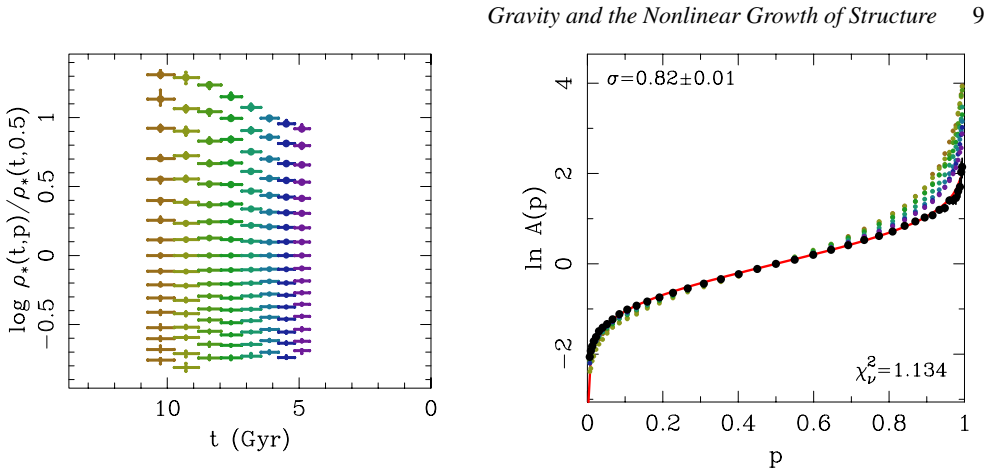
The paper claims that after a density fluctuation decouples from the Hubble expansion, the mean evolution of its overdensity is governed by the volume-averaged Lagrangian fluid equations, and that for the ensemble of mass parcels sharing an initial overdensity $\delta_p$ the result is $\langle D^2\delta/D\tau^2\rangle = \frac{3}{2}\Omega_M H_0^2 a^{-1}\delta_p^2$. Integrating once in time gives a mean growth rate proportional to $\delta_p^2(\tau-\tau_{nl})$, and integrating again gives the quadratic trajectory $\delta(\tau)-\delta(\tau_{nl}) \propto \delta_p^2(\tau-\tau_{nl})^2$, so $\alpha=2$ and $\beta=2$; underdense percentiles drain according to a mirrored law with an extra $(1+\delta_p)^2$ factor. The paper reports that fixed percentiles of the local stellar-mass density distribution in the CSI survey evolve with $\alpha = 1.98 \pm 0.04$ and $\beta = 2.01 \pm 0.11$, and that extrapolating each percentile back to the start of galaxy growth recovers a lognormal initial density distribution with $\sigma = 0.82 \pm 0.01$. These results are presented as the first exact, analytic description of nonlinear structure growth that extends to arbitrarily low redshift and as evidence that early lognormal fluctuations grew by gravitational accretion.
Load-bearing premise
The derivation hinges on assuming that the average expansion term within each group of mass parcels that began with the same initial density is the same as the average over all space, namely zero; if that conditional average is not zero, the predicted $\delta_0^2 t^2$ growth law does not follow.
Editorial extensions
If this is right
- Percentile-by-percentile density growth in the fully nonlinear regime is predictable from a closed algebraic form, so the growth of structure no longer needs to be treated as a purely numerical problem.
- Evolving observed density percentiles backwards recovers the initial lognormal spectrum with $\sigma = 0.82 \pm 0.01$, giving a direct empirical handle on the density field at the start of star formation.
- Because the derived form extends to arbitrarily low redshift, galaxy growth and the turnover in the cosmic star formation rate density can be modeled analytically rather than only through Monte Carlo techniques.
- The inferred Hurst parameter $H=1$ for accretion means the scatter around mean galaxy growth relations is itself correlated signal, so cross-sectional surveys should be analyzed distributionally rather than by tracking medians alone.
- Any additional physics, such as baryonic feedback or environmental effects, should enter as modified boundary or initial conditions, making measurements of $\alpha$ and $\beta$ a diagnostic for such physics.
Reading between the lines
- If the conditional-mean step at equation (6) survives scrutiny, the same volume-averaging trick may yield analytic growth laws for velocity statistics or higher-order density moments, not just percentile trajectories.
- Because the $\alpha=2$, $\beta=2$ law should hold for any tracer of the underlying density field, applying the same analysis to X-ray clusters, HI maps, or lensing maps would test whether baryonic tracers follow identical exponents or reveal feedback-induced deviations.
- The exponent pair ($\alpha,\beta$) is a redshift-independent benchmark; deviations measured in a particular percentile or scale could be converted into constraints on assembly bias or on the epoch of nonlinearity $z_{nl}$.
- A straightforward simulation test is to repeat the CSI percentile analysis on mock catalogs with full selection effects: recovering $\alpha = \beta = 2$ would close the loop, while any offset would quantify the systematic error budget of the measurement.
Signed reviews
Editorial analysis
A structured set of objections, weighed in public.
Referee Report
Summary. The paper claims a new analytic description of nonlinear structure growth: after overdense regions decouple from the Hubble expansion, fixed percentiles of the real-space matter density distribution should grow as δ(t) ∝ δ_0^α t^β with α = 2 and β = 2. This is derived in Section 2 by volume-averaging the Lagrangian fluid equations, and the prediction is tested against environmental densities measured from the Carnegie-Spitzer-IMACS Redshift Survey over 0.2 < z < 1.5, yielding α = 1.98 ± 0.04 and β = 2.01 ± 0.11.
Significance. If the derivation and measurement were both sound, the result would be significant: it would provide a simple analytic law for the growth of density percentiles into the nonlinear regime and would give the first direct observational confirmation of such a law. The paper also contains substantial empirical work: careful SED fitting, Monte Carlo tests of incompleteness corrections, Delaunay-based density estimation, and robustness checks over many redshift and mass binning choices. However, the theoretical core has two unproven and apparently incorrect steps, and the empirical validation is partly circular because the initial density distribution is inferred from the same data with the growth law already assumed. The paper's central claims are therefore not established.
major comments (4)
- [§2, Eq. (6)] The replacement of the conditional volume integral of ∇·u over parcels with initial overdensity Qδ(p) by the full-volume integral is asserted without support. In the linear growing mode, ∇·u/(aH) = -f δ with f ≈ Ω_m^0.55, so the conditional mean of ∇·u over parcels with δ(m, τ_nl) = δ_p is -aH f δ_p, not the global mean (zero for a periodic volume). At first order in δ_p, Eq. (6) therefore fails, and the '+1' term in Eq. (5) is not removed. Since Eq. (7) and the subsequent derivation all rest on this step, the quadratic growth law does not follow from the fluid equations as presented.
- [§2, Eqs. (8)–(9)] Taking the Lagrangian time derivative of the product δ (∇·u) in Eq. (8) produces two terms, but Eq. (9) retains only the term involving δ ∇·(Du/Dτ). The discarded term is (Dδ/Dτ)(∇·u) = -(1+δ)(∇·u)^2 by Eq. (1), which is nonzero and on nonlinear scales is generally comparable to the retained term. No argument is given for its vanishing. Without this additional and unjustified truncation, Eq. (11) is not derived.
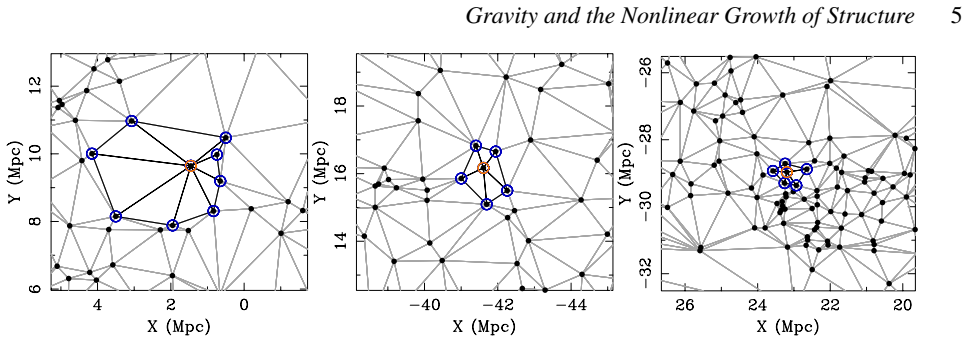
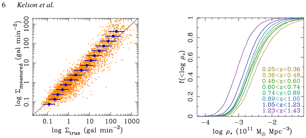
- [§6 and §7, Eqs. (16)–(17)] The empirical confirmation is partly circular. The initial lognormal A(p) = exp[σ Φ^{-1}(p)] is inferred from the same CSI percentile tracks in Section 6 after assuming β = 2, and σ is fitted. The relation B(p) ∝ [A(p)-1]^α is then compared with the data, but A(p) is constructed from those data. In addition, the free normalization γ in Eq. (17) absorbs the predicted prefactor C, so the agreement of α and β with (2, 2) tests only the shape of the growth law, not the quantitative normalization of Eq. (14). The reported posteriors therefore do not constitute an independent confirmation of the analytic derivation.
- [§2, Eq. (14)] The low-density branch of Eq. (14) is introduced through a brief chain-rule argument involving δ′ = ⟨ρ⟩/ρ − 1, but the derivation is not shown. In particular, the factor (1+δ_p)^2 and the statement about mass conservation in the p < 0.5 ensemble require a careful accounting of how parcels leave the percentile ensemble; as written, this part of the result is not established at the same level as the high-density branch.
minor comments (4)
- [§6, first paragraph] Typo: 'distrbution' should be 'distribution'.
- [§8, final paragraph] Typo: 'Eulerian' should be 'Eulerian'.
- [Throughout] A number of spelling errors appear: 'outlyers' should be 'outliers', 'correspondance' should be 'correspondence', and 'stricly' should be 'strictly'.
- [§7, Fig. 11 caption] The low-density percentiles with Φ^{-1}(p) < -1 are excluded from the fit, but the model curves are still shown for them using dashed lines; the text should state explicitly that those dashed curves are extrapolations, not fits.
Circularity Check
No circularity found: the §2 derivation does not use the CSI data or fitted parameters, and the empirical exponents α and β are free parameters in the final fit rather than constructions.
full rationale
The central derivation in §2 begins from the Lagrangian continuity equation, the momentum equation in the decoupled regime, and the Poisson equation (Eqs. 1–3); it does not import the CSI measurements, the fitted lognormal parameters, or any result from the authors' prior papers. The claimed scaling δ(t) ∝ δ0^2 t^2 is obtained by volume-averaging these fluid equations; it is not assumed as an input. Whether Eq. 6's conditional-averaging identity is valid is a mathematical correctness concern, not a circularity concern: a false step cannot make the conclusion identical to the premise by construction. In §6–7, the initial density distribution A(p) is inferred from the CSI percentile tracks, and then α, β, γ, and σ are treated as free parameters in Eq. 17 and marginalized over a four-dimensional grid. Since α and β are not fixed to 2 before the fit, the posterior estimates α = 1.98 ± 0.04 and β = 2.01 ± 0.11 are genuine measurements rather than forced values. The comparison of B(p) to [A(p)−1]^α is a test of a predicted functional relation between two empirically estimated quantities, analogous to a scaling-relation test; there is no statistical identity that forces the quadratic relation. The paper's self-citations to Kelson et al. (2014, 2016) appear in the SED-library construction and in the interpretative discussion of Hurst exponents; neither is load-bearing for the derivation of α = 2 and β = 2. Thus, no circular step meeting the evidentiary standard can be identified.
Assumptions & free parameters
free parameters (5)
- sigma (width of initial lognormal) =
0.82+/-0.01 in the first pass; marginalized in the final fit
- gamma (normalization of growth rate) =
order-unity nuisance, marginalized
- alpha (density-growth exponent) =
1.98+/-0.04
- beta (time-growth exponent) =
2.01+/-0.11
- z_nl (epoch of nonlinearity) =
10 (adopted)
assumptions (6)
- domain assumption After decoupling from the Hubble expansion, the momentum equation is Du/Dtau=-grad phi with no Hubble drag terms, and a is fixed at decoupling (Eqs 1-3).
- domain assumption Modes grow independently before nonlinearity, making the conditional volume integral of div u equal to the global volume average (Eq 6).
- ad hoc to paper Only one term survives the time derivative of the averaged product delta div u (Eqs 8-9).
- domain assumption Galaxy stellar mass density traces matter density in the mean on scales above individual halos.
- domain assumption The initial density distribution at the start of stellar mass growth is lognormal with unknown width sigma.
- domain assumption Fixed percentiles in cross-sectional density distributions can be modeled as evolving Lagrangian ensembles.
Cite this review
Pith. "Pith review of Gravity and the Nonlinear Growth of Structure in the Carnegie-Spitzer-IMACS Redshift Survey." pith.science (2026). https://pith.science/paper/6R2AJHNQ
@misc{pith2026190808952,
  author       = {Pith},
  title        = {Pith review of: Gravity and the Nonlinear Growth of Structure in the Carnegie-Spitzer-IMACS Redshift Survey},
  year         = {2026},
  howpublished = {\url{https://pith.science/paper/6R2AJHNQ}},
  note         = {Machine review of arXiv:1908.08952}
}
abstract
A key obstacle to developing a satisfying theory of galaxy evolution is the difficulty in extending analytic descriptions of early structure formation into full nonlinearity, the regime in which galaxy growth occurs. Extant techniques, though powerful, are based on approximate numerical methods whose Monte Carlo-like nature hinders intuition building. Here, we develop a new solution to this problem and its empirical validation. We first derive closed-form analytic expectations for the evolution of fixed percentiles in the real-space cosmic density distribution, {\it averaged over representative volumes observers can track cross-sectionally\}. Using the Lagrangian forms of the fluid equations, we show that percentiles in $\delta$---the density relative to the median---should grow as $\delta(t)\propto\delta_{0}^{\alpha}\,t^{\beta}$, where $\alpha\equiv2$ and $\beta\equiv2$ for Newtonian gravity at epochs after the overdensities transitioned to nonlinear growth. We then use 9.5 sq. deg. of Carnegie-Spitzer-IMACS Redshift Survey data to map {\it galaxy\} environmental densities over $0.2<z<1.5$ ($\sim$7 Gyr) and infer $\alpha=1.98\pm0.04$ and $\beta=2.01\pm0.11$---consistent with our analytic prediction. These findings---enabled by swapping the Eulerian domain of most work on density growth for a Lagrangian approach to real-space volumetric averages---provide some of the strongest evidence that a lognormal distribution of early density fluctuations indeed decoupled from cosmic expansion to grow through gravitational accretion. They also comprise the first exact, analytic description of the nonlinear growth of structure extensible to (arbitrarily) low redshift. We hope these results open the door to new modeling of, and insight-building into, the galaxy growth and its diversity in cosmological contexts.
Figures

Figures from the paper (5 more)




Reference graph
Works this paper leans on
-
[1]
Abramson, L. E., Gladders, M. D., Dressler, A., et al. 2015, ApJ, 801, L12
work page 2015
-
[2]
Abramson, L. E., Gladders, M. D., Dressler, A., et al. 2016, ApJ, 832, 7
work page 2016
-
[3]
Achitouv, I., Rasera, Y ., Sheth, R. K., & Corasaniti, P. S. 2013, Physical Review Letters, 111, 231303
work page 2013
-
[4]
S., Wechsler, R
Behroozi, P. S., Wechsler, R. H., & Conroy, C. 2013, ApJ, 770, 57
2013
-
[5]
J., Bower, R
Benson, A. J., Bower, R. G., Frenk, C. S., et al. 2003, ApJ, 599, 38
2003
-
[6]
Benson, A. J. 2014, MNRAS, 444, 2599
work page 2014
-
[7]
1992, New Insights into the Universe, 65
Bertschinger, E. 1992, New Insights into the Universe, 65
work page 1992
- [8]
Show all 46 references
-
[9]
R., Faber, S
Blumenthal, G. R., Faber, S. M., Primack, J. R., & Rees, M. J. 1984, Nature, 311, 517
1984
-
[10]
R., Cole, S., Efstathiou, G., & Kaiser, N
Bond, J. R., Cole, S., Efstathiou, G., & Kaiser, N. 1991, ApJ, 379, 440
1991
-
[11]
Bouchet, F. R. 1996, Dark Matter in the Universe, 565
1996
-
[12]
L., Blanton, M
Coil, A. L., Blanton, M. R., Burles, S. M., et al. 2011, ApJ, 741, 8
2011
-
[13]
S., Navarro, J
Cole, S., Aragon-Salamanca, A., Frenk, C. S., Navarro, J. F., & Zepf, S. E. 1994, MNRAS, 271, 781
1994
-
[14]
1991, MNRAS, 248, 1
Coles, P., & Jones, B. 1991, MNRAS, 248, 1
1991
-
[15]
C., Yan, R., Dickinson, M., et al
Cooper, M. C., Yan, R., Dickinson, M., et al. 2012, MNRAS, 425, 2116
2012
-
[16]
1980, ApJ, 236, 351
Dressler, A. 1980, ApJ, 236, 351
1980
-
[17]
2011, PASP, 123, 288
Dressler, A., Bigelow, B., Hare, T., et al. 2011, PASP, 123, 288
2011
-
[18]
D., Abramson, L
Dressler, A., Kelson, D. D., Abramson, L. E., et al. 2016, ApJ, 833, 251
2016
-
[19]
D., & Abramson, L
Dressler, A., Kelson, D. D., & Abramson, L. E. 2018, ApJ, 869, 152 Driver S.P. & Robotham A.S.G., 2010, MNRAS, 407, 2131
2018
-
[20]
D., Oemler, A., Dressler, A., et al
Gladders, M. D., Oemler, A., Dressler, A., et al. 2013, ApJ, 770, 64
2013
-
[21]
Kauffmann, G., White, S. D. M., & Guiderdoni, B. 1993, MNRAS, 264, 201
1993
- [22]
- [23]
-
[24]
2016, MNRAS, 457, 4340
Klypin, A., Yepes, G., Gottlöber, S., Prada, F., & Heß, S. 2016, MNRAS, 457, 4340
2016
-
[25]
2018, MNRAS, 474, 5206 Le Fevre, O., Vettolani, G., Maccagni, D., et al
Knebe, A., Stoppacher, D., Prada, F., et al. 2018, MNRAS, 474, 5206 Le Fevre, O., Vettolani, G., Maccagni, D., et al. 2003, Proc. SPIE, 173
2018
-
[26]
J., Le Fevre, O., Hammer, F., & Crampton, D
Lilly, S. J., Le Fevre, O., Hammer, F., & Crampton, D. 1996, ApJ, 460, L1
1996
-
[27]
1995, ApJ, 455, 7
Ma, C.-P., & Bertschinger, E. 1995, ApJ, 455, 7
1995
-
[28]
Ma, C.-P., & Fry, J. N. 2000, ApJ, 543, 503
2000
-
[29]
C., Dickinson, M
Madau, P., Ferguson, H. C., Dickinson, M. E., et al. 1996, MNRAS, 283, 1388
1996
-
[30]
2018, ARA&A, 56, 393
Mandelbaum, R. 2018, ARA&A, 56, 393
2018
-
[31]
B., & van Ness, J
Mandelbrot, B. B., & van Ness, J. W. 1968, SIAM Review, 10, 422
1968
-
[32]
B., & Wallis, J
Mandelbrot, B. B., & Wallis, J. R. 1969, Water Resources Research, 5, 228
1969
-
[33]
Q., Hahn, G
Meeker, W. Q., Hahn, G. J., & Escobar, L. A., 2017,Statistical Intervals: A Guide for Practitioners and Researchers, John Wiley & Sons
2017
-
[34]
P., Naab, T., & White, S
Moster, B. P., Naab, T., & White, S. D. M. 2013, MNRAS, 428, 3121
2013
-
[35]
R., et al
Moutarde, F., Alimi, J.-M., Bouchet, F. R., et al. 1991, ApJ, 382, 377
1991
-
[36]
G., Weiner, B
Noeske, K. G., Weiner, B. J., Faber, S. M., et al. 2007, ApJ, 660, L43
2007
-
[37]
2004, ApJ, 608, 647
Ohta, Y ., Kayo, I., & Taruya, A. 2004, ApJ, 608, 647
2004
-
[38]
G., et al
Oemler, A., Jr., Dressler, A., Gladders, M. G., et al. 2013, ApJ, 770, 63
2013
-
[39]
Peebles, P. J. E. 1967, ApJ, 147, 859
1967
-
[40]
Peebles, P. J. E. 1974, A&A, 32, 391
1974
-
[41]
J., Kovaˇc, K., et al
Peng, Y .-j., Lilly, S. J., Kovaˇc, K., et al. 2010, ApJ, 721, 193
2010
-
[42]
J., Renzini, A., & Carollo, M
Peng, Y .-j., Lilly, S. J., Renzini, A., & Carollo, M. 2012, ApJ, 757, 4 Planck Collaboration, Ade, P. A. R., Aghanim, N., et al. 2015, arXiv:1502.01589
2012 arXiv
-
[43]
H., & Schechter, P
Press, W. H., & Schechter, P. 1974, ApJ, 187, 425
1974
-
[44]
2018, A&A, 609, A84
Scodeggio, M., Guzzo, L., Garilli, B., et al. 2018, A&A, 609, A84
2018
-
[45]
and Lorensen, B
Shroeder, W., Martin, K. and Lorensen, B. 2002, The Visualization Toolkit, 3rd Edition. Kitware Inc., New York. van der Burg, R. F. J., Muzzin, A., Hoekstra, H., et al. 2013, A&A, 557, A15
2002
-
[46]
2011, ApJ, 735, 32 Zel’dovich, Y
Wang, X., Neyrinck, M., Szapudi, I., et al. 2011, ApJ, 735, 32 Zel’dovich, Y . B. 1970, A&A, 5, 84 This paper has been typeset from a TEX/LATEX file prepared by the author. MNRAS 000, 1–13 (0000)
2011
Reviewed August 14, 2026 · model on record in the stance chip above.
Discussion (0). Continue with ORCID to comment.