REVIEW 4 major objections 5 minor 34 references
Well-posedness study of a non-linear hyperbolic-parabolic coupled system applied to image speckle reduction
T0 review · 4 major / 5 minor · reviewed 2026-08-14 · deepseek-v4-flash
Pith's one-line read The paper proves that a coupled telegraph-diffusion equation for image intensity and a parabolic equation for edge strength admit exactly one weak solution, and that the solution preserves the intensity range.
desk verdict A novel coupled hyperbolic-parabolic despeckling model with a plausible well-posedness theorem whose proof leans heavily on an unverified companion preprint; the numerics are tuned best-case comparisons. read the letter →
The pith
A machine-rendered reading of the paper's core claim, the machinery that carries it, and where it could break.
The reading
What carries the argument
The carrying object is the diffusion coefficient $g(I,u)=\frac{s^\alpha}{1+s^\alpha}\cdot\frac{1}{1+|u_\xi|^\beta}$, where $s=|I_\xi|/M_{I_\xi}$ is the Gaussian-smoothed intensity normalized by its spatial maximum and $u_\xi$ is the smoothed edge-strength variable. In the linearized problem the coefficient is frozen at $(\overline I,\overline u)$, and the proof needs the bounds $0<\kappa\le \overline g\le 1$ and $|\overline g_t|\le C$ from (2.3); these turn the second-order telegraph equation into a coercive linear problem solvable by classical Galerkin approximation. Schauder's fixed-point theorem (a compactness-based principle producing fixed points of continuous maps on convex sets) transfers linearized solvability back to the nonlinear system. The uniqueness argument is carried by the Lipschitz continuity of $h$ and the positive lower bound on $I$, which together control the difference between two solutions through a Gronwall inequality.
What would settle it
Start from an $H^2$ image with a small positive minimum and a narrow valley; if the Gaussian convolution $G_\xi * I$ reaches zero during the evolution, the uniform lower bound $\kappa>0$ in (2.3) is violated and the theorem's fixed-point domain cannot be built.
Extended reading notes
Core claim
The central claim is Theorem 2.1: the system (1.2)--(1.4), with $\gamma=\iota=\nu=1$, admits a unique weak solution $(I,u) \in W(0,T)$ in the sense of Definition 2.1 whenever $I_0 \in H^2$ has a positive infimum and $h:\mathbb{R}_+\to\mathbb{R}_+$ is bounded and Lipschitz with $0\le h\le 1$. The proof picks a bounded, convex, weakly compact set of candidate pairs and, for any fixed candidate $(\overline I,\overline u)$, solves the linearized telegraph equation and the linearized edge equation. The linearized solutions satisfy uniform estimates, so the solution map is weakly continuous and Schauder's fixed-point theorem produces a pair $(I,u)$ that solves the original coupled system. Uniqueness is shown by taking the difference of two weak solutions, testing against integrated test functions, and running a step-by-step Gronwall argument from $0$ to $T$. Lemma 2.3 adds that any weak solution preserves the initial intensity bounds, $0<\rho \le I(t,x)\le \varrho$.
Load-bearing premise
The argument depends on an estimate, taken from a companion preprint rather than proved here, that the smoothed image intensity stays bounded away from zero and that the diffusion coefficient changes at a controlled rate; if that estimate fails, the linearized problem and the fixed-point construction are not defined.
Editorial extensions
If this is right
- The model is well-posed as an evolution equation: once the noisy image and edge-response function are fixed, the despeckling trajectory is uniquely determined in the stated solution class.
- The proven boundedness of the solution means intensities cannot leave the interval $[\rho,\varrho]$ during denoising, so repeated filtering cannot produce out-of-range gray values.
- The hypotheses on $h$ cover the concrete choice $h(\theta)=\epsilon+\min\{\theta^2,K\}$ used in the experiments, so the numerical tests fall within the scope of the theorem.
- The proof pattern (freeze coefficients, solve linearly, apply a fixed-point principle) can be reused for other coupled hyperbolic-parabolic image models with bounded Lipschitz edge detectors.
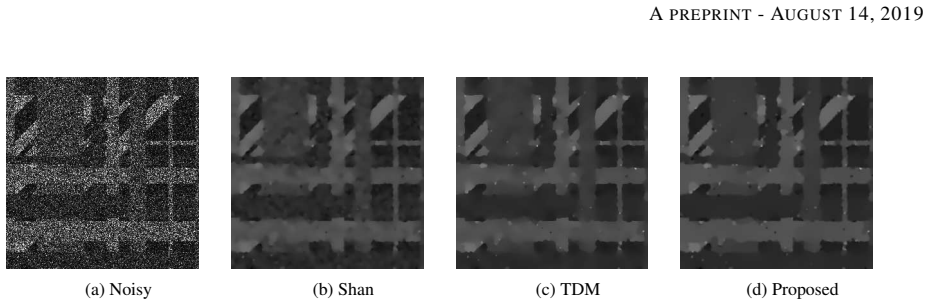
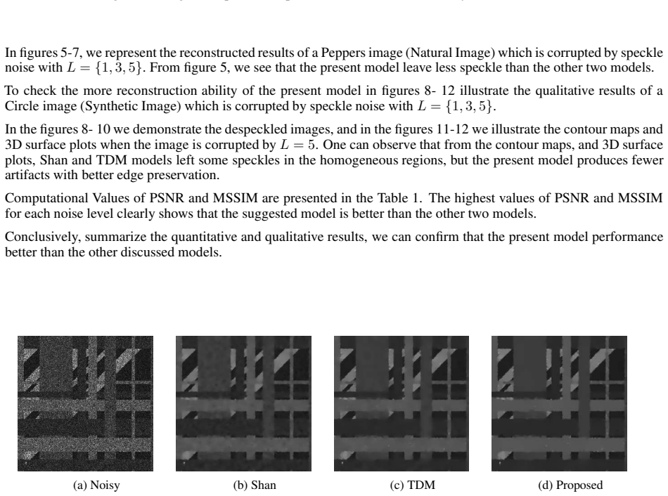
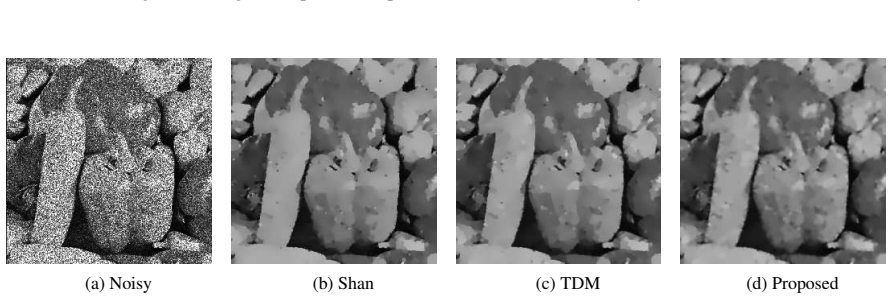
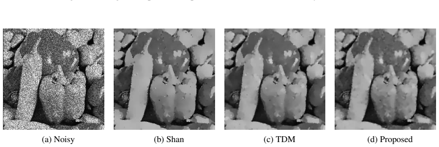
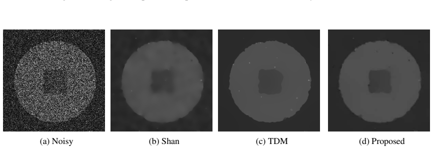
- The comparison tables show the proposed model achieving the highest PSNR and MSSIM values on all three test images at all three speckle levels, supporting the paper's claim of better edge preservation.
Reading between the lines
- Beyond the paper: if the lower bound $\kappa>0$ is genuinely needed, the model's well-posedness is most fragile for nearly black images; an initial image whose Gaussian-smoothed intensity approaches zero would leave the theorem's hypothesis and should be probed as a stress test.
- Beyond the paper: the numerical section uses the explicit scheme (3.1)--(3.2) without proving its stability or convergence, so linking the discrete iterates to the weak solution is an open next step.
- Beyond the paper: the same coupling framework could accommodate learned or data-driven edge maps, since any bounded, Lipschitz replacement for $h(|\nabla I_\xi|)$ would inherit the well-posedness argument provided the coefficient bounds still hold.
- Beyond the paper: the step-by-step Gronwall uniqueness argument suggests that the small-time uniqueness technique generalizes to other coupled parabolic-hyperbolic systems in image processing.
Signed reviews
Editorial analysis
A structured set of objections, weighed in public.
Referee Report
Summary. The manuscript proposes a coupled hyperbolic-parabolic PDE system, equations (1.2)-(1.4), for speckle reduction: a telegraph-diffusion equation for the intensity I coupled to a reaction-diffusion equation for an edge variable u. The main theoretical result is Theorem 2.1, which asserts existence and uniqueness of weak solutions in a space W(0,T) under assumptions A.1-A.2, proved via a Schauder fixed-point argument on a linearized problem. The paper also reports numerical experiments on three gray-level test images, comparing PSNR and MSSIM values with two prior models, and concludes that the proposed model performs better.
Significance. If the well-posedness proof is made fully self-contained, the paper would provide a rigorous foundation for a novel coupled hyperbolic-parabolic despeckling model, which is a potentially useful contribution to PDE-based image processing. The numerical section is clearly organized, includes explicit finite-difference discretizations, and compares against two recent models with tables of PSNR/MSSIM values. However, the central analytic proof depends essentially on the authors' companion preprint [22] for several key estimates, and no machine-checked proofs or code are supplied. The claimed numerical advantage is modest and is obtained with an oracle stopping criterion, so the practical claim should be read cautiously.
major comments (4)
- [Section 2.2, Eq. (2.3)] The proof of Theorem 2.1 rests on the assertion that for every (¯I, ¯u) in B_{M1,M2}, the coefficient ¯g satisfies 0 < κ ≤ ¯g ≤ 1 and |¯g_t| ≤ C. This is not proved in the paper; it is attributed to 'a similar argument as in the proof of [22, Claim 2.1].' The lower bound κ > 0 is needed for the linearized problem to be uniformly parabolic and for the Galerkin estimates, while the bound on ¯g_t requires time-regularity of the diffusion coefficient and control of ∂_t ¯I and ∂_t ¯u. Neither estimate is derived here, so the existence part of Theorem 2.1 is conditional on external companion results.
- [Section 2.3, definition of W0 and map P] The Schauder map is stated as P: W0 → W0, but the paper does not prove that the solution (I,u) of the linearized problem (2.1)-(2.2) satisfies the defining properties of W0, in particular the lower bound 0 < ρ ≤ I(t,x). Lemma 2.3, which gives a two-sided bound for weak solutions, is stated after Theorem 2.1 and for solutions of the nonlinear system, so it cannot be invoked before a fixed point is known to exist. Without a proof that P preserves W0, the fixed-point argument cannot close.
- [Section 2.3, weak continuity of P] The claimed weak continuity of P requires passing to the limit in the nonlinear coefficient ¯g_k := |G_ξ*w_k|^α / ((M^{w_k}_ξ)^α + |G_ξ*w_k|^α) · 1/(1+|G_ξ*v_k|^β). The argument lists strong L2 and a.e. convergences for quantities involving G_ξ*w_k and G_ξ*v_k, but does not prove convergence of the maxima M^{w_k}_ξ = max_{x∈Ω} |G_ξ*w_k(t,x)|. Weak convergence in W0 only provides compactness subsequences, and the conclusion that the entire sequence P(w_k,v_k) converges to P(w,v) requires additional justification. This gap is load-bearing for the fixed-point step.
- [Section 2.3, uniqueness proof after Eq. (2.10)] The uniqueness proof is not self-contained: inequality (2.10) is imported from [22, Section 3.3] without derivation, and the estimate ||(g_{I1,u1} - g_{I2,u2})(t)||_{L∞} ≤ C(||I(t)||^α_{L2} + ||u(t)||_{L2}) is asserted using the positive lower bound ρ of the two solutions. But for arbitrary weak solutions the lower bound is not yet available unless Lemma 2.3 is proved independently. Additionally, the Gronwall step after (2.12) writes 'u(s) ≤ ...' where the norm of u(s) is intended; this should be written as ||u(s)||_{L2}^2.
minor comments (5)
- [Section 2.2] There is a typo: 'revels' should be 'reveals' in the sentence following equation (2.3).
- [Section 2.3] In the paragraph before equation (2.10), 'in the sence of distribution' should read 'in the sense of distribution.'
- [Section 3] The stopping criterion is described as 'when the best PSNR value for the restored image is reached,' which requires access to the original clean image. A practical despeckling algorithm would need a data-dependent stopping rule; this should be stated explicitly.
- [Section 3, Table 1] The right half of Table 1 reports parameter values but the column labels do not clearly indicate which model the parameters belong to; the reader has to infer from the order of the models in the text. A clearer table header would help.
- [References [21], [22]] References [21] and [22] are cited with nonstandard URLs beginning with https://128.84.21.199/abs/; these should be updated to standard arXiv links.
Circularity Check
Theorem 2.1's proof delegates its key coefficient bounds, fixed-point estimates, and uniqueness inequality to the same authors' companion preprint [22], making the well-posedness claim conditional on a load-bearing self-citation chain.
-
self citation load bearing
[Section 2.2, equation (2.3)]
"Since ( ¯I, ¯u) ∈ B M1,M 2 , a similar argument as in the proof of [22, Claim 2.1] revels that i) 0 < κ ≤ ¯g ≤ 1 , ii) |¯gt| ≤ C , (2.3)"
This is the ellipticity and time-regularity bound for the diffusion coefficient g_bar in the linearized problem. It is not proved here; it is delegated to Claim 2.1 of [22], a companion arXiv preprint by the same three authors, which is not machine-checked, not code-reproduced, and not externally falsified. The entire Galerkin step and the definition of the Schauder map P on W0 depend on this bound: without 0 < kappa <= g_bar, (2.1) is not uniformly elliptic. The strong well-posedness claim in Theorem 2.1 therefore inherits its key quantitative input from an overlapping self-citation rather than from a derivation in this paper.
-
self citation load bearing
[Section 2.2, proof of Lemma 2.2]
"Since ‖¯ut‖L∞(0,T ;L2) ≤ C‖I0‖H1 , by following computations as in Sudeb at el. [22, Lemma 3.2] , one can show the validation of the estimates a) and b) of Lemma 2.2."
Estimates (a) and (b) are precisely the bounds that keep P(w,v) inside W0 and give weak compactness for the fixed-point argument. The paper supplies no computation for them; it points to Lemma 3.2 of the same authors' companion preprint. The estimate for (c) is sketched, but (a) and (b) are load-bearing and deferred. This makes the existence half of Theorem 2.1 conditional on an overlapping self-citation rather than on an argument in the text.
2 more flagged steps
-
self citation load bearing
[Section 2.3, uniqueness proof around (2.10)-(2.12)]
"Then, by using a similar argument as in [22, Section 3.3], we obtain 12 ‖I(s)‖2L2 + ∫s0 ‖I(t)‖2L2 dt + C‖w(s)‖2H1 ≤ ˜Cs ‖w(s)‖2H1 + C∫s0 (‖w(t)‖2H1 + ‖I(t)‖2L2 + ‖u(t)‖2L2) dt ."
The uniqueness inequality and the Gronwall step that closes the proof are not derived; the paper says to repeat [22, Section 3.3]. The auxiliary lower bound for gI1,u1 is again taken 'like in (2.3)', which itself comes from [22]. Thus the uniqueness half of Theorem 2.1 reduces to the same companion preprint by the same authors rather than to an independent argument in the present text.
-
self citation load bearing
[Section 2.3, Lemma 2.3]
"For any weak solution (I, u) of (1.2)-(1.4), we next show the boundedness of I under the assumption that initial image I0 has a finite upper bound, whose proof follows from the proof of [22, Lemma 3.3]."
Although this boundedness lemma is stated after the existence proof and is not used in the fixed-point argument, it is presented as a result of the paper, and its proof is entirely a reference to [22, Lemma 3.3], again a result from the same authors' companion preprint. It contributes to the general pattern that the paper's mathematical content is heavily carried by self-citation.
full rationale
The paper does not commit the cleanest form of circularity: no equation in the text is defined in terms of the theorem's conclusion, and the numerical PSNR/MSSIM claims are empirical comparisons rather than predictions fitted from the model. However, Theorem 2.1 is not self-contained. The key coefficient bound (2.3), the W0-norm estimates in Lemma 2.2(a,b), the uniqueness inequality, and Lemma 2.3 are all referred to the same authors' companion preprint [22] (arXiv:1908.01147), which is not machine-checked, has no supplied code, and is not externally validated. These deferred estimates are exactly the quantitative inputs that make the linearized problem uniformly elliptic and that keep the Schauder map P inside W0; without them the Galerkin step and weak-continuity argument do not close. The paper therefore falls under the self-citation load-bearing pattern: the central well-posedness claim is conditional on an overlapping-authority chain rather than derived here. Because the proof also contains some independent structure, such as the sketch for the u-estimate, the compactness subsequences, and the Gronwall framework, the circularity is partial rather than total, so the score is 6. The numerical comparison is not itself circular, though it is weakened by per-image and per-noise retuning of parameters.
Assumptions & free parameters
free parameters (5)
- Model parameters alpha, beta, gamma, nu, iota =
Varies per image and noise level in Table 1 (right); e.g., (1.5,1.8,10,1,1) for Circle at L=1
- Stopping iteration (oracle PSNR) =
Not reported; chosen as the best-PSNR iteration
- Gaussian width xi in G_xi =
xi = 1
- Time step tau and spatial step h =
tau = 0.2, h = 1
- Edge-response parameters epsilon and K in h(theta) = epsilon + min{theta^2, K} =
K = (max gray level)^2, epsilon small
assumptions (6)
- standard math Linear well-posedness: the classical Galerkin method yields a unique weak solution of the linearized system (2.1)-(2.2).
- standard math Schauder's fixed point theorem applies to the weakly continuous map P on the weakly compact convex set W0.
- standard math Compact Sobolev embedding theorems (Aubin-Lions type) yield the strong convergences used in passing to the limit.
- domain assumption A.1: the initial image I0 lies in H2 and has a strictly positive lower bound rho.
- domain assumption A.2: the edge-response function h is bounded and Lipschitz, with 0 <= h <= 1.
- ad hoc to paper The evolving intensity stays strictly positive (0 < rho <= I) and the linearized coefficient obeys 0 < kappa <= g <= 1 with |g_t| <= C.
invented entities (1)
-
Edge variable u(t,x) governed by u_t = h(|grad I_xi|) - u + (nu^2/2) Laplace u
Cite this review
Pith. "Pith review of Well-posedness study of a non-linear hyperbolic-parabolic coupled system applied to image speckle reduction." pith.science (2026). https://pith.science/paper/6RQ43AIU
@misc{pith2026190802653,
  author       = {Pith},
  title        = {Pith review of: Well-posedness study of a non-linear hyperbolic-parabolic coupled system applied to image speckle reduction},
  year         = {2026},
  howpublished = {\url{https://pith.science/paper/6RQ43AIU}},
  note         = {Machine review of arXiv:1908.02653}
}
read the original abstract
In this article, we consider a non-linear hyperbolic-parabolic coupled system based on telegraph diffusion framework applied to image despeckling. A separate equation is used to calculate the edge variable, which improves the quality of the despeckled images. A well-posedness result of the proposed coupled system is settled via Schauder's fixed point theorem. Numerical experiments are reported to illustrate the effectiveness of the proposed model, with recently developed models, over a set of gray level test images contaminated by speckle noise.
Figures


Figures from the paper (9 more)



Reference graph
Works this paper leans on
-
[14]
Circuits, Systems, and Signal Proces sing pp
Jain, S.K., Ray, R.K., Bhavsar, A.: A nonlinear coupled diffusion system for image despeckling and application to ultrasound images. Circuits, Systems, and Signal Proces sing pp. 1-30 (2018)
work page 2018
-
[28]
Boundary V alue Problems 2016(1), 187 (2016) 12 A PREPRINT - A UGUST 14, 2019
Sun, J., Y ang, J., Sun, L.: A class of hyperbolic-parabo lic coupled systems applied to image restoration. Boundary V alue Problems 2016(1), 187 (2016) 12 A PREPRINT - A UGUST 14, 2019
work page 2016
-
[22]
Majee, S., Ray, R.K., Majee, A.K.: A gray level indicato r-based regularized telegraph diffusion equation applied to image despeckling, a preprint arXiv https://128.84.21.199/abs/1908.01147, (2019)
work page Pith review arXiv 2019
-
[1]
Adam, Sobolev spaces, in: Pure and Applied Mathematic s Series of Monographs and Textbooks, V ol
R. Adam, Sobolev spaces, in: Pure and Applied Mathematic s Series of Monographs and Textbooks, V ol. 65, Academic Press, Inc., New Y ork, San Francisco, London„ 1975
work page 1975
-
[2]
IEEE Geoscience and remote sensing magazine 1(3), 6 -35 (2013) A PREPRINT - A UGUST 14, 2019
Argenti, F., Lapini, A., Bianchi, T., Alparone, L.: A tut orial on speckle reduction in synthetic aperture radar images. IEEE Geoscience and remote sensing magazine 1(3), 6 -35 (2013) A PREPRINT - A UGUST 14, 2019
work page 2013
-
[3]
SIAM Journal on Applied Mathe- matics 68(4), 925-946 (2008)
Aubert, G., Aujol, J.F.: A variational approach to remov ing multiplicative noise. SIAM Journal on Applied Mathe- matics 68(4), 925-946 (2008)
work page 2008
-
[4]
Nonlinear Analysis: Real World Applications 11(1), 253-26 1 (2010)
Cao, Y ., Yin, J., Liu, Q., Li, M.: A class of nonlinear para bolic-hyperbolic equations applied to image restoration. Nonlinear Analysis: Real World Applications 11(1), 253-26 1 (2010)
2010
-
[5]
Applied soft computing 8(2), 919-927 (2008)
Chaira, T., Ray, A.: A new measure using intuitionistic f uzzy set theory and its application to edge detection. Applied soft computing 8(2), 919-927 (2008)
work page 2008
Show all 34 references
-
[6]
In: Abstract and Applied Analysis , vol
Dong, G., Guo, Z., Wu, B.: A convex adaptive total variati on model based on the gray level indicator for multi- plicative noise removal. In: Abstract and Applied Analysis , vol. 2013. Hindawi Publishing Corporation (2013)
2013
-
[7]
Ultrasound Research Laboratory p
Dutt, V .: Statistical analysis of ultrasound echo envel ope. Ultrasound Research Laboratory p. 181 (1995)
1995
-
[8]
Evans, L.: Partial Differential Equations, in: Graduat e Studies in Mathematics, vol. 19. American Mathematical Society, Providence, Rhode Island (1998)
1998
-
[9]
Gonzalez, R.C., Woods, R.E.: Digital image processing ( 2002)
2002
-
[10]
AEU-International Journal of Electronics and Com munications 69(9), 1291-1296 (2015)
Hao, Y ., Xu, J., Li, S., Zhang, X.: A variational model ba sed on split bregman method for multiplicative noise removal. AEU-International Journal of Electronics and Com munications 69(9), 1291-1296 (2015)
2015
-
[11]
EURASIP Journal on image and video processing 2010(1), 1 (2010)
Huang, L.L., Xiao, L., Wei, Z.H.: Multiplicative noise removal via a novel variational model. EURASIP Journal on image and video processing 2010(1), 1 (2010)
2010
-
[12]
In: Information Systems Design and Intelligent Applications, pp
Jain, S.K., Ray, R.K.: Edge detectors based telegraph t otal variational model for image filtering. In: Information Systems Design and Intelligent Applications, pp. 119-126. Springer (2016)
2016
-
[13]
IETE Technical Review pp
Jain, S.K., Ray, R.K.: Non-linear diffusion models for despeckling of images: achievements and future chal- lenges. IETE Technical Review pp. 1-17 (2019)
2019
-
[15]
In: Inter- national Conference on Pattern Recognition and Mach ine Intelligence, pp
Jidesh, P ., Bini, A.: A complex diffusion driven approa ch for removing data-dependent multiplicative noise. In: Inter- national Conference on Pattern Recognition and Mach ine Intelligence, pp. 284-289. Springer (2013)
2013
-
[16]
IEEE Trans - actions on Information Technology in Biomedicine 4(4), 298 -305 (2000)
Jin, J.S.,Wang, Y ., Hiller, J.: An adaptive nonlinear d iffusion algorithm for filtering medical images. IEEE Trans - actions on Information Technology in Biomedicine 4(4), 298 -305 (2000)
2000
-
[17]
Journal of Mathematical Analysis and Applications 362(2), 415-426 (2010)
Jin, Z., Y ang, X.: Analysis of a new variational model fo r multiplicative noise removal. Journal of Mathematical Analysis and Applications 362(2), 415-426 (2010)
2010
-
[18]
Journal of Math- ematical Imaging and Vision 39(1), 62-74 (2011)
Jin, Z., Y ang, X.: A variational model to remove the mult iplicative noise in ultrasound images. Journal of Math- ematical Imaging and Vision 39(1), 62-74 (2011)
2011
-
[19]
Journal of Visual Communi- cation and Image Representation 36, 187-198 (2016 )
Liu, M., Fan, Q.: A modified convex variational model for multiplicative noise removal. Journal of Visual Communi- cation and Image Representation 36, 187-198 (2016 )
2016
-
[20]
Nonlinear Analysis: Real World Applications 14(5), 2046-2058 (2013)
Liu, Q., Li, X., Gao, T.: A nondivergence p-laplace equa tion in a removing multiplicative noise model. Nonlinear Analysis: Real World Applications 14(5), 2046-2058 (2013)
2013
-
[21]
Majee, S., Jain, S.K., Ray, R.K., Majee, A.K.: A fuzzy ed ge detector driven telegraph total variation model for image despeckling, a preprint arXiv https://128.84.21.199/abs/1908.01134, (2019)
2019 arXiv
-
[23]
Pattern Analysis and Machine Intel- ligence, IEEE Transactions on 12(7), 629-639 (1990)
Perona, P ., Malik, J.: Scale-space and edge detection u sing anisotropic diffusion. Pattern Analysis and Machine Intel- ligence, IEEE Transactions on 12(7), 629-639 (1990)
1990
-
[24]
In: Image Analysis and Processing, 2007
Ratner, V ., Zeevi, Y .Y .: Image enhancement using elastic manifolds. In: Image Analysis and Processing, 2007. ICIAP 2007. 14th International Conference on, pp. 769-774. IEEE (2007)
2007
-
[25]
In: Geometric Level Set Methods in Imaging, Vision, and Graphics, pp
Rudin, L., Lions, P .L., Osher, S.: Multiplicative deno ising and deblurring: Theory and algorithms. In: Geometric Level Set Methods in Imaging, Vision, and Graphics, pp. 103- 119. Springer (2003)
2003
-
[26]
Journal of Mathe- matical Imaging and Vision pp
Shan, X., Sun, J., Guo, Z.: Multiplicative noise remova l based on the smooth diffusion equation. Journal of Mathe- matical Imaging and Vision pp. 1-17 (2019)
2019
-
[27]
SIAM Journal on Imaging Sciences 1(3), 294-321 (2008)
Shi, J., Osher, S.: A nonlinear inverse scale space meth od for a convex multiplicative noise model. SIAM Journal on Imaging Sciences 1(3), 294-321 (2008)
2008
-
[29]
Image Processing, IEEE Transactions on 1 3(4), 600-612 (2004)
Wang, Z., Bovik, A.C., Sheikh, H.R., Simoncelli, E.P .: Image quality assessment: from error visibility to struc- tural similarity. Image Processing, IEEE Transactions on 1 3(4), 600-612 (2004)
2004
-
[30]
Mathematical Problems in Engineering 2014 (2014)
Y ang, Y .Q., Zhang, C.Y .: Kernel based telegraph-diffu sion equation for image noise removal. Mathematical Problems in Engineering 2014 (2014)
2014
-
[31]
IEEE Transactions on image processing 11(11), 1260-1270 (2002)
Y u, Y ., Acton, S.T.: Speckle reducing anisotropic diff usion. IEEE Transactions on image processing 11(11), 1260-1270 (2002)
2002
-
[32]
Sign al Processing 107, 368-377 (2015)
Zhang, W ., Li, J., Y ang, Y .: Spatial fractional telegraph equation for image structure preserving denoising. Sign al Processing 107, 368-377 (2015)
2015
-
[33]
IEEE Tra nsactions on Image Processing 24(1), 249-260 (2015)
Zhou, Z., Guo, Z., Dong, G., Sun, J., Zhang, D., Wu, B.: A d oubly degenerate diffusion model based on the gray level indicator for multiplicative noise removal. IEEE Tra nsactions on Image Processing 24(1), 249-260 (2015)
2015
-
[34]
Journal of Nonlinear Science 28(2), 443-470 (2018 ) 13
Zhou, Z., Guo, Z., Zhang, D., Wu, B.: A nonlinear diffusi on equation-based model for ultrasound speckle noise removal. Journal of Nonlinear Science 28(2), 443-470 (2018 ) 13
2018
Reviewed August 14, 2026 · model on record in the stance chip above.
Discussion (0). Continue with ORCID to comment.