REVIEW 2 major objections 5 minor 26 references
Computational method for probability distribution on recursive relationships in financial applications
T0 review · 2 major / 5 minor · reviewed 2026-08-14 · deepseek-v4-flash
Pith's one-line read A backward-recursive convolution formula numerically gives the full conditional distribution of any sum of increments of a one-dimensional Markov process, covering densities, hedging errors, Asian options, and hypothesis tests.
desk verdict A competent, clearly written extension of a known recursive convolution method to several finance applications, but the advertised high accuracy outruns the numerical error analysis. read the letter →
The pith
A machine-rendered reading of the paper's core claim, the machinery that carries it, and where it could break.
The reading
What carries the argument
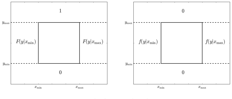
The central object is the conditional cumulative distribution function $F_n(y|x_n)$ of the remaining sum after time $n$; it is what the recursion propagates. The key identity is (4), $F_n(y|x_n)=\int_{\mathbb{R}} F_{n+1}(y-h(x_n,x_{n+1})|x_{n+1}) f(x_{n+1}|x_n)\,dx_{n+1}$, together with the terminal condition (5); differentiating in $y$ gives the density recursion (6). The numerical procedure discretizes state and value grids, uses interpolation to retrieve shifted values, assigns $0$ or $1$ for CDFs (or $0$ for densities) outside the $y$-range, and clamps to the boundary state when $x_{n+1}$ escapes the $x$-grid, with the paper arguing that the transition density is small there; the $y$-range is expanded adaptively as the support grows.
What would settle it
Run the recursion for the CIR model, where the true transition density has a closed form, using the paper's truncated state grid, and compare the computed density of $Y=X_N-X_0$ to the exact density; then repeat with a wider state grid. If the computed density changes materially with the grid width, the boundary-state approximation is not negligible and the claimed high accuracy fails in that setting.
Extended reading notes
Core claim
The paper claims that the conditional distribution of $Y=\sum_{i=1}^N h(X_{i-1},X_i)$ for a one-dimensional Markov process can be built by backward induction, and that its discrete approximation has high accuracy. Writing $F_n(y|x_n)$ for the conditional CDF of the remaining sum $\sum_{i=n+1}^N h(X_{i-1},X_i)$ given $X_n=x_n$, the paper derives $F_n(y|x_n)=\int_{\mathbb{R}} F_{n+1}(y-h(x_n,x_{n+1})|x_{n+1}) f(x_{n+1}|x_n)\,dx_{n+1}$, with the terminal condition $F_{N-1}(y|x_{N-1})=\mathbb{P}(y\ge h(x_{N-1},X_N)|x_{N-1})$. Differentiating both sides in $y$ yields the same recursion for conditional densities. The paper verifies the recursion on CIR, CEV, stochastic volatility, GARCH, variance-gamma hedging, Asian-option, and skewness-test examples, and notes that the computational cost is comparable to a Fourier-transform method while avoiding the final inverse transform.
Load-bearing premise
The method's claimed accuracy rests on the assumption that values of the next state outside the chosen state grid occur with small probability, so the boundary-state approximation used there contributes negligible error; no error bound is provided for this extrapolation.
Editorial extensions
If this is right
- For any one-dimensional Markov process with a computable transition density, the same recursion produces the full conditional density of the discrete-time sum, making models without closed-form densities (CEV, stochastic volatility, GARCH) numerically tractable.
- The hedging-error distribution can be obtained for both delta and minimum-variance strategies under exponential variance-gamma dynamics, giving a deterministic counterpart to simulation histograms.
- Arithmetic Asian option prices are recovered under risk-neutral transition densities by choosing $h(x_{i-1},x_i)=x_i/N$ or rescaling the distribution, with no closed-form pricing formula needed.
- For skewness tests on jump-diffusion returns, the recursion computes critical values and power curves directly from the law of $(\Delta R)^3$, avoiding normal approximations to the test statistic.
- The per-time-step cost is proportional to the product of the grid sizes ($N_x N_y N_z$), comparable to the Fourier characteristic-function approach, and the method avoids the final inverse transform.
Reading between the lines
- The recurrence is a distribution-valued dynamic program, so the same backward convolution applies to any additive functional of a Markov chain, suggesting occupation-time functionals, barrier hitting probabilities, and drawdown distributions as natural next applications.
- Because the only stochastic input is the transition density, accuracy will be governed by how well truncated grids capture the tail of that density; for heavy-tailed Lévy increments the fixed-grid clamping is the first place to test, and an adaptive or transformed state grid could restore accuracy where the current extrapolation fails.
- The scale-invariance remark implies a concrete efficiency gain: for homogeneous models one can fix $x_0=1$, compute the distribution of $Y/x_0$, and rescale, effectively reducing the state dimension in pricing applications.
Signed reviews
Editorial analysis
A structured set of objections, weighed in public.
Referee Report
Summary. The paper proposes a backward recursive numerical method for computing the conditional cumulative distribution function or density of Y = sum_{i=1}^N h(X_{i-1}, X_i) for a one-dimensional Markov process X. The recursion, given in Eqs. (4)-(6), expresses the conditional law of the remaining sum at step n as an integral of the law at step n+1 against the transition density. The authors describe a numerical implementation with an adaptive y-grid and reference rules outside the grid, then apply the method to CIR and CEV densities, stochastic-volatility integrated variance, GARCH variance and return distributions, variance-gamma delta-hedging and minimum-variance hedging errors, arithmetic Asian option prices, and a skewness test for a jump-diffusion model. The paper claims that numerical experiments show the method has high accuracy.
Significance. The central recursive identity in Eqs. (4)-(6) is correct and is derived cleanly from the Markov property; it provides a parameter-free deterministic alternative to Monte Carlo for one-dimensional state processes, and the scale-invariant reduction in Remark 1 is useful. The breadth of applications is a strength, and the paper includes an algorithm description with a code link, which aids reproducibility. The main weakness is that the claimed 'high accuracy' is not supported by a formal error analysis, and the numerical boundary treatment for out-of-grid states is justified only heuristically. The validation is mostly against Monte Carlo simulations that use the same transition densities, so systematic grid-truncation bias may be shared and masked. If the boundary issue is addressed with quantitative error bounds or convincing convergence studies, the method would be a solid contribution.
major comments (2)
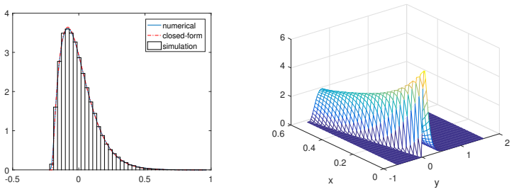
- [§2.2, 'Referencing previous function'] A second major issue is that the validation does not isolate the boundary error. The only independent check is the CIR closed-form comparison in Section 3.1.1 and Figure 2; Figures 5-10 compare the numerical densities against Monte Carlo histograms that use the same transition densities and, in all likelihood, the same grid truncation. Any systematic bias from the boundary extrapolation is therefore shared by both methods and is not visible in the comparisons. The claim in the abstract that the method 'has high accuracy' is thus not established for regimes with substantial transition mass away from the current state. I request convergence studies with respect to N_x, N_y, N_z, the tolerance, and especially the x-range, together with at least one additional independent benchmark beyond the CIR example, before the general accuracy claim can be accepted.
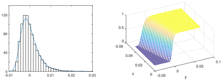
- [§3.5, skewness test] The jump-diffusion example is not fully specified. The section gives parameters λ = 10, σ_J = 0.01, μ_J = 0, and σ = 0.1975, but it does not state the time step δt, the observation horizon, the number of terms N in the sum for the test statistic, or the explicit transition density f(x_{n+1}|x_n) used in the recursion. Without these, Figure 11 cannot be reproduced and the accuracy of the critical values and power curve cannot be assessed. Please provide the complete specification of the transition density and the discretization parameters.
minor comments (5)
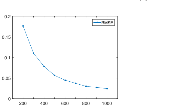
- [Figure 3] The quantity labeled 'Global error' is not defined; please specify the error metric, the densities being compared, and the domain of integration.
- [Algorithm 1] The algorithm uses non-standard symbols '⊿' and '≁'; please replace them with explicit and standard notation for assignment, function evaluation, and convergence testing.
- [§2.3] In the Fourier-transform comparison, the notation f(x_n, x_{n-1}) should be a conditional density f(x_n|x_{n-1}), and the arguments of h appear reversed in one place; please correct these typos.
- [Remark 1] The scale-invariance condition is stated as a property of X alone, but the relation g_n(y|x_n) = x_n g_n(y/x_n|1) also imposes a condition on the function h; please state the precise condition on h under which the reduction is valid.
- [§2.2, 'Adaptive meshing'] Because the number of y-grid points is fixed while the range [y_min, y_max] changes dynamically, the step size Δy changes at every backward step; the effect of this on interpolation error should be discussed or tested.
Circularity Check
No significant circularity: the recursive convolution formula follows directly from the Markov property, and the numerical validations test the integration scheme rather than renaming fitted inputs as predictions.
full rationale
The central derivation, Eqs. (4)-(6), is a direct application of the law of total expectation to the Markov process X: F_n(y|x_n) equals the integral of F_{n+1}(y-h(x_n,x_{n+1})|x_{n+1}) against the transition density f(x_{n+1}|x_n), with the terminal condition Eq. (5). This is a mathematical identity for the conditional distribution of Y = sum h(X_{i-1}, X_i), not an input assumed into the conclusion. No parameter is fitted to a subset of data and then predicted; the comparisons with the CIR closed form, Monte Carlo histograms, and Asian option simulations are consistency checks of the numerical integration. The self-citations (Park et al. 2016, Lee 2014) are contextual: the paper explicitly states Park et al. used "the same framework" and extends it, but the convolution identity is not justified by those citations. The only flagged limitation is in Section 2.2, where x_{n+1} outside [x_min, x_max] is assigned F_{n+1}(y|x_max) or F_{n+1}(y|x_min) because the transition density is "relatively small" there; this is a numerical accuracy and error-bound concern, not a circular step, since it is a discretization heuristic rather than a premise from which the claimed distribution is derived. Accordingly, no circular step is exhibited and the score is 0.
Assumptions & free parameters
free parameters (1)
- Numerical discretization parameters (N_x, N_y, N_z, tolerance) =
Varies by example; e.g., CIR: N_y=1000 intervals, epsilon=1e-8
assumptions (5)
- domain assumption The underlying process X is Markov and has transition densities f(x_{n+1}|x_n).
- domain assumption The transition densities f(x_{n+1}|x_n) are integrable and the relevant integrals converge.
- standard math Differentiation under the integral sign and interchange of integrals are valid, so Eq. (6) follows from Eq. (4).
- ad hoc to paper Extrapolation outside the numerical grid introduces negligible error: F_{n+1}=0 or 1 outside the y-range, and F_{n+1}(·|x_min) or F_{n+1}(·|x_max) outside the x-range.
- domain assumption For the CIR and CEV examples, the Euler-Maruyama Gaussian increment is an adequate approximation of the true transition density.
Cite this review
Pith. "Pith review of Computational method for probability distribution on recursive relationships in financial applications." pith.science (2026). https://pith.science/paper/6SDYZUA7
@misc{pith2026190804959,
  author       = {Pith},
  title        = {Pith review of: Computational method for probability distribution on recursive relationships in financial applications},
  year         = {2026},
  howpublished = {\url{https://pith.science/paper/6SDYZUA7}},
  note         = {Machine review of arXiv:1908.04959}
}
read the original abstract
In quantitative finance, it is often necessary to analyze the distribution of the sum of specific functions of observed values at discrete points of an underlying process. Examples include the probability density function, the hedging error, the Asian option, and statistical hypothesis testing. We propose a method to calculate such a distribution, utilizing a recursive method, and examine it using various examples. The results of the numerical experiment show that our proposed method has high accuracy.
Figures
Figures from the paper (8 more)




Reference graph
Works this paper leans on
-
[1]
Barndorff-Nielsen, O. E. (2002). Econometric analysis of realized volatility and its use in estimating stochastic volatility models. Journal of the Royal Statistical Society: Series B (Statistical Methodology) , 64:253--280
work page 2002
-
[2]
Bollerslev, T. (1986). Generalized autoregressive conditional heteroskedasticity. Journal of econometrics , 31:307--327
work page 1986
-
[3]
Breeden, D. T. and Litzenberger, R. H. (1978). Prices of state-contingent claims implicit in option prices. Journal of business , pages 621--651
work page 1978
-
[4]
Broadie, M. and Kaya, \"O . (2006). Exact simulation of stochastic volatility and other affine jump diffusion processes. Operations Research , 54:217--231
work page 2006
-
[5]
Carr, P. and Madan, D. (1999). Option valuation using the fast F ourier transform. Journal of computational finance , 2:61--73
work page 1999
-
[6]
Choe, G. H. and Lee, K. (2014). High moment variations and their application. Journal of Futures Markets , 34:1040--1061
2014
-
[7]
Christoffersen, P., Heston, S., and Jacobs, K. (2006). Option valuation with conditional skewness. Journal of Econometrics , 131:253--284
work page 2006
-
[8]
Christoffersen, P., Jacobs, K., and Mimouni, K. (2010). Volatility dynamics for the S & P 500: evidence from realized volatility, daily returns, and option prices. Review of Financial Studies , 23:3141--3189
work page 2010
Show all 26 references
-
[9]
Cont, R. (2001). Empirical properties of asset returns: stylized facts and statistical issues. Quantitative Finance , 1:223--236
2001
-
[10]
Cont, R., Tankov, P., and Voltchkova, E. (2007). Hedging with options in models with jumps. In Stochastic analysis and applications , pages 197--217. Springer
2007
-
[11]
C., Ingersoll Jr, J
Cox, J. C., Ingersoll Jr, J. E., and Ross, S. A. (1985). A theory of the term structure of interest rates. Econometrica , 53:385--407
1985
-
[12]
Cox, J. C. and Ross, S. A. (1976). The valuation of options for alternative stochastic processes. Journal of financial economics , 3:145--166
1976
-
[13]
Fama, E. F. (1965). The behavior of stock-market prices. The Journal of Business , 38:34--105
1965
-
[14]
and Sondermann, D
F \"o llmer, H. and Sondermann, D. (1986). Hedging of non-redundant contingent claims. In Contributions to Mathematical Economics: In Honor of G \'e rard Debreu , pages 205--224. North Holland
1986
-
[15]
R., Schwert, G
French, K. R., Schwert, G. W., and Stambaugh, R. F. (1987). Expected stock returns and volatility. Journal of Financial Economics , 19:3--29
1987
-
[16]
Harvey, C. R. and Siddique, A. (2000). Conditional skewness in asset pricing tests. Journal of Finance , 55:1263--1295
2000
-
[17]
Heston, S. L. (1993). A closed-form solution for options with stochastic volatility with applications to bond and currency options. Review of Financial Studies , 6:327--343
1993
-
[18]
Kemna, A. G. and Vorst, A. (1990). A pricing method for options based on average asset values. Journal of Banking & Finance , 14:113--129
1990
-
[19]
and Litzenberger, R
Kraus, A. and Litzenberger, R. H. (1976). Skewness preference and the valuation of risk assets. Journal of Finance , 31:1085--1100
1976
-
[20]
Lee, K. (2014). Recursive formula for arithmetic Asian option prices. Journal of Futures Markets , 34:220--234
2014
-
[21]
Lee, K. (2016). Probabilistic and statistical properties of moment variations and their use in inference and estimation based on high frequency return data. Studies in Nonlinear Dynamics & Econometrics , 20:19--36
2016
-
[22]
B., Carr, P
Madan, D. B., Carr, P. P., and Chang, E. C. (1998). The variance gamma process and option pricing. European finance review , 2:79--105
1998
-
[23]
and Rutkowski, M
Musiela, M. and Rutkowski, M. (2006). Martingale methods in financial modelling , volume 36. Springer Science & Business Media
2006
-
[24]
Park, M., Lee, K., and Choe, G. H. (2016). Distribution of discrete time delta-hedging error via a recursive relation. East Asian Journal on Applied Mathematics , 6:314--336
2016
-
[25]
Sepp, A. (2012). An approximate distribution of delta-hedging errors in a jump-diffusion model with discrete trading and transaction costs. Quantitative Finance , 12:1119--1141
2012
-
[26]
V e c e r, J. (2002). Unified Asian pricing. Risk , 15:113--116
2002
Reviewed August 14, 2026 · model on record in the stance chip above.
Discussion (0). Continue with ORCID to comment.